Python Fundamentals

Overview

Teaching: 20 min
Exercises: 10 min

Questions

• What basic data types can I work with in Python?

• How can I create a new variable in Python?

• How do I use a function?

• Can I change the value associated with a variable after I create it?

Objectives

• Assign values to variables.

Variables

Any Python interpreter can be used as a calculator:

3 + 5 * 4

23

This is great but not very interesting. To do anything useful with data, we need to assign its value to a variable. In Python, we can assign a value to a variable, using the equals sign =. For example, we can track the weight of a patient who weighs 60 kilograms by assigning the value 60 to a variable weight_kg:

weight_kg = 60

From now on, whenever we use weight_kg, Python will substitute the value we assigned to it. In layperson’s terms, a variable is a name for a value.

In Python, variable names:

• can include letters, digits, and underscores
• cannot start with a digit
• are case sensitive.

This means that, for example:

• weight0 is a valid variable name, whereas 0weight is not
• weight and Weight are different variables

Types of data

Python knows various types of data. Three common ones are:

• integer numbers
• floating point numbers, and
• strings.

In the example above, variable weight_kg has an integer value of 60. If we want to more precisely track the weight of our patient, we can use a floating point value by executing:

weight_kg = 60.3

To create a string, we add single or double quotes around some text. To identify and track a patient throughout our study, we can assign each person a unique identifier by storing it in a string:

patient_id = '001'

Using Variables in Python

Once we have data stored with variable names, we can make use of it in calculations. We may want to store our patient’s weight in pounds as well as kilograms:

weight_lb = 2.2 * weight_kg

We might decide to add a prefix to our patient identifier:

patient_id = 'inflam_' + patient_id

Built-in Python functions

To carry out common tasks with data and variables in Python, the language provides us with several built-in functions. To display information to the screen, we use the print function:

print(weight_lb)
print(patient_id)

132.66
inflam_001

When we want to make use of a function, referred to as calling the function, we follow its name by parentheses. The parentheses are important: if you leave them off, the function doesn’t actually run! Sometimes you will include values or variables inside the parentheses for the function to use. In the case of print, we use the parentheses to tell the function what value we want to display. We will learn more about how functions work and how to create our own in later episodes.

We can display multiple things at once using only one print call:

print(patient_id, 'weight in kilograms:', weight_kg)

inflam_001 weight in kilograms: 60.3

We can also call a function inside of another function call. For example, Python has a built-in function called type that tells you a value’s data type:

print(type(60.3))
print(type(patient_id))

<class 'float'>
<class 'str'>

Moreover, we can do arithmetic with variables right inside the print function:

print('weight in pounds:', 2.2 * weight_kg)

weight in pounds: 132.66

The above command, however, did not change the value of weight_kg:

print(weight_kg)

60.3

To change the value of the weight_kg variable, we have to assign weight_kg a new value using the equals = sign:

weight_kg = 65.0
print('weight in kilograms is now:', weight_kg)

weight in kilograms is now: 65.0

Variables as Sticky Notes

A variable in Python is analogous to a sticky note with a name written on it: assigning a value to a variable is like putting that sticky note on a particular value.

Using this analogy, we can investigate how assigning a value to one variable does not change values of other, seemingly related, variables. For example, let’s store the subject’s weight in pounds in its own variable:

# There are 2.2 pounds per kilogram
weight_lb = 2.2 * weight_kg
print('weight in kilograms:', weight_kg, 'and in pounds:', weight_lb)

weight in kilograms: 65.0 and in pounds: 143.0

Similar to above, the expression 2.2 * weight_kg is evaluated to 143.0, and then this value is assigned to the variable weight_lb (i.e. the sticky note weight_lb is placed on 143.0). At this point, each variable is “stuck” to completely distinct and unrelated values.

Let’s now change weight_kg:

weight_kg = 100.0
print('weight in kilograms is now:', weight_kg, 'and weight in pounds is still:', weight_lb)

weight in kilograms is now: 100.0 and weight in pounds is still: 143.0

Since weight_lb doesn’t “remember” where its value comes from, it is not updated when we change weight_kg.

Check Your Understanding

What values do the variables mass and age have after each of the following statements? Test your answer by executing the lines.

mass = 47.5
age = 122
mass = mass * 2.0
age = age - 20

Solution

`mass` holds a value of 47.5, `age` does not exist
`mass` still holds a value of 47.5, `age` holds a value of 122
`mass` now has a value of 95.0, `age`'s value is still 122
`mass` still has a value of 95.0, `age` now holds 102

Sorting Out References

Python allows you to assign multiple values to multiple variables in one line by separating the variables and values with commas. What does the following program print out?

first, second = 'Grace', 'Hopper'
third, fourth = second, first
print(third, fourth)

Solution

Hopper Grace

Seeing Data Types

What are the data types of the following variables?

planet = 'Earth'
apples = 5
distance = 10.5

Solution

print(type(planet))
print(type(apples))
print(type(distance))

<class 'str'>
<class 'int'>
<class 'float'>

Key Points

• Basic data types in Python include integers, strings, and floating-point numbers.

• Use variable = value to assign a value to a variable in order to record it in memory.

• Variables are created on demand whenever a value is assigned to them.

• Use print(something) to display the value of something.

• Built-in functions are always available to use.

Analyzing some wave-height data

Overview

Teaching: 40 min
Exercises: 20 min

Questions

• How can I process tabular data files in Python?

Objectives

• Explain what a library is and what libraries are used for.

• Import a Python library and use the functions it contains.

• Read tabular data from a file into a program.

• Select individual values and subsections from data.

• Perform operations on arrays of data.

Words are useful, but what’s more useful are the sentences and stories we build with them. Similarly, while a lot of powerful, general tools are built into Python, specialized tools built up from these basic units live in libraries that can be called upon when needed.

Loading data into Python

To begin processing the wavedata, we need to load it into Python. We can do that using a library called NumPy, which stands for Numerical Python. In general, you should use this library when you want to do fancy things with lots of numbers, especially if you have matrices or arrays. To tell Python that we’d like to start using NumPy, we need to import it:

import numpy

Importing a library is like getting a piece of lab equipment out of a storage locker and setting it up on the bench. Libraries provide additional functionality to the basic Python package, much like a new piece of equipment adds functionality to a lab space. Just like in the lab, importing too many libraries can sometimes complicate and slow down your programs - so we only import what we need for each program.

Once we’ve imported the library, we can ask the library to read our data file for us:

numpy.loadtxt(fname='wavesmonthly.csv', delimiter=',', skiprows=1)

array([[1.979e+03, 1.000e+00, 3.788e+00],
       [1.979e+03, 2.000e+00, 3.768e+00],
       [1.979e+03, 3.000e+00, 4.774e+00],
       ...,
       [2.015e+03, 1.000e+01, 3.046e+00],
       [2.015e+03, 1.100e+01, 4.622e+00],
       [2.015e+03, 1.200e+01, 5.048e+00]])

The expression numpy.loadtxt(...) is a function call that asks Python to run the function loadtxt which belongs to the numpy library. The dot notation in Python is used most of all as an object attribute/property specifier or for invoking its method. object.property will give you the object.property value, object_name.method() will invoke on object_name method.

As an example, John Smith is the John that belongs to the Smith family. We could use the dot notation to write his name smith.john, just as loadtxt is a function that belongs to the numpy library.

numpy.loadtxt has two parameters: the name of the file we want to read and the delimiter that separates values on a line. These both need to be character strings (or strings for short), so we put them in quotes. Notice that we also had to tell NumPy to skip the first row, which contains the column titles.

Since we haven’t told it to do anything else with the function’s output, the notebook displays it. In this case, that output is the data we just loaded. By default, only a few rows and columns are shown (with ... to omit elements when displaying big arrays). Note that, to save space when displaying NumPy arrays, Python does not show us trailing zeros, so 1.0 becomes 1..

Our call to numpy.loadtxt read our file but didn’t save the data in memory. To do that, we need to assign the array to a variable. In a similar manner to how we assign a single value to a variable, we can also assign an array of values to a variable using the same syntax. Let’s re-run numpy.loadtxt and save the returned data:

data = numpy.loadtxt(fname='wavesmonthly.csv', delimiter=',', skiprows=1)

This statement doesn’t produce any output because we’ve assigned the output to the variable data. If we want to check that the data have been loaded, we can print the variable’s value:

print(data)

[[1.979e+03 1.000e+00 3.788e+00]
 [1.979e+03 2.000e+00 3.768e+00]
 [1.979e+03 3.000e+00 4.774e+00]
 ...
 [2.015e+03 1.000e+01 3.046e+00]
 [2.015e+03 1.100e+01 4.622e+00]
 [2.015e+03 1.200e+01 5.048e+00]]

Now that the data are in memory, we can manipulate them. First, let’s ask what type of thing data refers to:

print(type(data))

<class 'numpy.ndarray'>

The output tells us that data currently refers to an N-dimensional array, the functionality for which is provided by the NumPy library. These data correspond to sea wave height. Each row is a monthly average, and the columns are their associated dates and values.

Data Type

A Numpy array contains one or more elements of the same type. The type function will only tell you that a variable is a NumPy array but won’t tell you the type of thing inside the array. We can find out the type of the data contained in the NumPy array.

print(data.dtype)

float64

This tells us that the NumPy array’s elements are floating-point numbers.

With the following command, we can see the array’s shape:

print(data.shape)

(444, 3)

The output tells us that the data array variable contains 444 rows (sanity check: 37 years of 12 months = 37 * 12 = 444) and 3 columns (year, month, and datapoint). When we created the variable data to store our wave data, we did not only create the array; we also created information about the array, called members or attributes. This extra information describes data in the same way an adjective describes a noun. data.shape is an attribute of data which describes the dimensions of data. We use the same dotted notation for the attributes of variables that we use for the functions in libraries because they have the same part-and-whole relationship.

If we want to get a single number from the array, we must provide an index in square brackets after the variable name, just as we do in math when referring to an element of a matrix. Our wave data has two dimensions, so we will need to use two indices to refer to one specific value:

print('first value in data:', data[0, 2])

first value in data: 3.788

print('middle value in data:', data[222, 2])

middle value in data: 2.446

The expression data[222, 2] accesses the element at row 222, column 2. While this expression may not surprise you, using data[0, 2] to get the 3rd column in the 1st row might. Programming languages like Fortran, MATLAB and R start counting at 1 because that’s what human beings have done for thousands of years. Languages in the C family (including C++, Java, Perl, and Python) count from 0 because it represents an offset from the first value in the array (the second value is offset by one index from the first value). This is closer to the way that computers represent arrays (if you are interested in the historical reasons behind counting indices from zero, you can read Mike Hoye’s blog post). As a result, if we have an M×N array in Python, its indices go from 0 to M-1 on the first axis and 0 to N-1 on the second. It takes a bit of getting used to, but one way to remember the rule is that the index is how many steps we have to take from the start to get the item we want.

In the Corner

What may also surprise you is that when Python displays an array, it shows the element with index [0, 0] in the upper left corner rather than the lower left. This is consistent with the way mathematicians draw matrices but different from the Cartesian coordinates. The indices are (row, column) instead of (column, row) for the same reason, which can be confusing when plotting data.

Slicing data

An index like [222, 2] selects a single element of an array, but we can select whole sections as well. For example, we can select the wavedata for the first year like this:

print(data[0:12, 0:3])

[[1.979e+03 1.000e+00 3.788e+00]
 [1.979e+03 2.000e+00 3.768e+00]
 [1.979e+03 3.000e+00 4.774e+00]
 [1.979e+03 4.000e+00 2.818e+00]
 [1.979e+03 5.000e+00 2.734e+00]
 [1.979e+03 6.000e+00 2.086e+00]
 [1.979e+03 7.000e+00 2.066e+00]
 [1.979e+03 8.000e+00 2.236e+00]
 [1.979e+03 9.000e+00 3.322e+00]
 [1.979e+03 1.000e+01 3.512e+00]
 [1.979e+03 1.100e+01 4.348e+00]
 [1.979e+03 1.200e+01 4.628e+00]]

The slice 0:12 means, “Start at index 0 and go up to, but not including, index 12”. Again, the up-to-but-not-including takes a bit of getting used to, but the rule is that the difference between the upper and lower bounds is the number of values in the slice.

We don’t have to start slices at 0:

print(data[12:24, 1:3])

[[ 1.     3.666]
 [ 2.     4.326]
 [ 3.     3.522]
 [ 4.     3.18 ]
 [ 5.     1.954]
 [ 6.     1.72 ]
 [ 7.     1.86 ]
 [ 8.     1.95 ]
 [ 9.     3.11 ]
 [10.     3.78 ]
 [11.     3.474]
 [12.     5.28 ]]

We also don’t have to include the upper and lower bound on the slice. If we don’t include the lower bound, Python uses 0 by default; if we don’t include the upper, the slice runs to the end of the axis, and if we don’t include either (i.e., if we use ‘:’ on its own), the slice includes everything:

first_year = data[:12, 2:]
print('data from first year is:')
print(first_year)

The above example selects rows 0 through 11 and columns 2 through to the end of the array (which in this case is only the last column).

data from first year is:
[[3.788]
 [3.768]
 [4.774]
 [2.818]
 [2.734]
 [2.086]
 [2.066]
 [2.236]
 [3.322]
 [3.512]
 [4.348]
 [4.628]]

Analyzing data

NumPy has several useful functions that take an array as input to perform operations on its values. If we want to find the average wave height for all months on all years, for example, we can ask NumPy to compute data’s mean value:

print(numpy.mean(data))

668.9611876876877

mean is a function that takes an array as an argument. Given that our array contains the dates as well as data, with numbers relating to years and months, taking the mean of the whole array doesn’t really make much sense - we don’t expect to see 600 metre high waves!

We can use slicing to calculate the correct mean:

print(numpy.mean(data[:,2]))

3.383563063063063

Not All Functions Have Input

Generally, a function uses inputs to produce outputs. However, some functions produce outputs without needing any input. For example, checking the current time doesn’t require any input.

import time
print(time.ctime())

Sat Mar 26 13:07:33 2016

For functions that don’t take in any arguments, we still need parentheses (()) to tell Python to go and do something for us.

Let’s use three other NumPy functions to get some descriptive values about the wave heights. We’ll also use multiple assignment, a convenient Python feature that will enable us to do this all in one line.

maxval, minval, stdval = numpy.max(data[:,2]), numpy.min(data[:,2]), numpy.std(data[:,2])

print('Max wave height:', maxval)
print('Min wave height:', minval)
print('Wave height standard deviation:', stdval)

Here we’ve assigned the return value from numpy.max(data[:,2]) to the variable maxval, the value from numpy.min(data[:,2]) to minval, and so on. Note that we used maxval, rather than just max - it’s not good practice to use variable names that are the same as Python keywords or fuction names.

Max wave height: 6.956
Min wave height: 1.496
Wave height standard deviation: 1.1440155050316319

Mystery Functions in IPython

How did we know what functions NumPy has and how to use them? If you are working in IPython or in a Jupyter Notebook, there is an easy way to find out. If you type the name of something followed by a dot, then you can use tab completion (e.g. type numpy. and then press Tab) to see a list of all functions and attributes that you can use. After selecting one, you can also add a question mark (e.g. numpy.cumprod?), and IPython will return an explanation of the method! This is the same as doing help(numpy.cumprod). Similarly, if you are using the “plain vanilla” Python interpreter, you can type numpy. and press the Tab key twice for a listing of what is available. You can then use the help() function to see an explanation of the function you’re interested in, for example: help(numpy.cumprod).

What about NaNs?

In real datasets, particularly ones which come from observational data, it’s quite common for some values to be missing. There are various strategies to deal with missing values; one of which is to give them a value that would be clearly wrong (e.g. -1 for a temperature column with units in
Kelvin, or 999 for a missing latitude or longitude value). However, the issue with this is that we would need to check for these values before calculating any summary statistic.

Instead, we can use NumPy’s NaN (“not a number”) value, which will tell NumPy that these are values that need to be dealt with in a special manner. NumPy also provides various functions to help deal with NaNs. However, we can’t use NumPy’s normal statistical functions on any array that contains a NaN, as this returns a NaN:

data = numpy.array([[1,2,3],[1,numpy.NaN,3],[1,2,3]])
numpy.mean(data)

nan

Instead, we need to use the NumPy function nanmean:

data = numpy.array([[1,2,3],[1,numpy.NaN,3],[1,2,3]])
numpy.nanmean(data)

2.0

If, at a later date, we’d like to replace all the NaNs with a sensible numerical value (e.g. the mean of the column), NumPy also provides functions that can help with this

What happens if the shape of the data is not convenient for us to do some of our analysis? With this waveheight dataset, the data is a time-series, but it’s not very easy to calculate things like average monthly temperature. To do that, we’ll need to reshape it. Numpy allows us to do that relatively easily:

reshaped_data = numpy.reshape(data[:,2], [37,12]) # reshape the data to form a 2D array of year by month

We now have a 2D array of data using, where each row is a year, and each column represents a month:

print("The shape of the reshaped data is:")
print(numpy.shape(reshaped_data))

The shape of the reshaped data is:
(37, 12)

We can verify that nothing about the data has changed:

print(f"The maximum value of the reshaped data is: {numpy.max(reshaped)}")
print(f"The minimum value of the reshaped data is: {numpy.min(reshaped)}")
print(f"The standard deviation of the reshaped data is: {numpy.std(reshaped)}")

The maximum value of the reshaped data is: 6.956
The minimum value of the reshaped data is: 1.496
The standard deviation of the reshaped data is: 1.1440155050316319

Printing text

Earlier on in the episide, we just printed text in one print statement, and output in a different print statement. However, in the last example, we printed text and output in the same print statement. Python has several ways to achieve this, but the way we just used is the most modern, and is formally called “Formatted string literals”, but more commonly called “f-strings”. We need to prefix the string with the letter ‘f’, but then anything within curly brackets is interpreted by python:

name = 'Jon'
city = 'Cardiff'
print(f"Hello, My name is {name} and I live in {city}.")

F-strings can be used in most cases where we want to print outut with text, but there are some advanced edge-cases where the more verbose string formatting still needs to be used

We can now look variations in some summary statistics, such as the maximum wave height per month, or average height per year more easily. One way to do this is to create a new temporary array of the data we want, then ask it to do the calculation:

year_0 = reshaped_data[0,:] # 0 on the first axis (rows), everything on the second (columns)
print(f"maximum wave height for year 0: {numpy.max(year_0)}")

maximum wave height for year 0: 4.774

Everything in a line of code following the ‘#’ symbol is a comment that is ignored by Python. Comments allow programmers to leave explanatory notes for other programmers or their future selves.

What if we need the maximum wave height for each month over all years (as in the next diagram on the left) or the average for each day (as in the diagram on the right)? As the diagram below shows, we want to perform the operation across an axis:

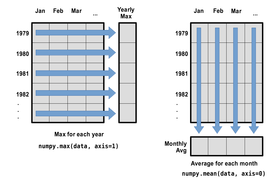
To support this functionality, most array functions allow us to specify the axis we want to work on. If we ask for the average across axis 0 (rows in our 2D example), we get:

print(numpy.mean(reshaped_data, axis=0))

[6.956 6.074 6.184 5.838 4.882 4.754 4.648 4.688 5.064 5.032 5.15  6.044]

As a quick check, we can ask this array what its shape is:

print(numpy.mean(data, axis=0).shape)

(12,)

The expression (12,) tells us we have an N×1 vector, so this is the average wave height per month for all years. If we average across axis 1 (columns in our 2D example), we get:

print(numpy.mean(reshaped_data, axis=1))

[3.34       3.15183333 3.29866667 3.53366667 3.448      3.23016667
 2.99383333 3.51133333 2.96066667 3.20316667 3.62116667 5.1915
 3.28816667 3.529      3.523      3.66866667 3.314      2.99916667
 3.45983333 3.16783333 3.413      3.3435     3.031      3.29366667
 3.138      3.29716667 3.3185     3.24966667 3.4135     3.42866667
 3.168      2.78816667 3.61366667 3.2725     3.32766667 3.2765
 4.385     ]

which is the average wave height per month across all years.

Slicing Strings

A section of an array is called a slice. We can take slices of character strings as well:

element = 'oxygen'
print('first three characters:', element[0:3])
print('last three characters:', element[3:6])

first three characters: oxy
last three characters: gen

What is the value of element[:4]? What about element[4:]? Or element[:]?

Solution

oxyg
en
oxygen

What is element[-1]? What is element[-2]?

Solution

n
e

Given those answers, explain what element[1:-1] does.

Solution

Creates a substring from index 1 up to (not including) the final index, effectively removing the first and last letters from ‘oxygen’

How can we rewrite the slice for getting the last three characters of element, so that it works even if we assign a different string to element? Test your solution with the following strings: carpentry, clone, hi.

Solution

element = 'oxygen'
print('last three characters:', element[-3:])
element = 'carpentry'
print('last three characters:', element[-3:])
element = 'clone'
print('last three characters:', element[-3:])
element = 'hi'
print('last three characters:', element[-3:])

last three characters: gen
last three characters: try
last three characters: one
last three characters: hi

Thin Slices

The expression element[3:3] produces an empty string, i.e., a string that contains no characters. If data holds our array of wave data, what does data[3:3, 4:4] produce? What about data[3:3, :]?

Solution

array([], shape=(0, 0), dtype=float64)
array([], shape=(0, 40), dtype=float64)

Stacking Arrays

Arrays can be concatenated and stacked on top of one another, using NumPy’s vstack and hstack functions for vertical and horizontal stacking, respectively.

import numpy

A = numpy.array([[1,2,3], [4,5,6], [7, 8, 9]])
print('A = ')
print(A)

B = numpy.hstack([A, A])
print('B = ')
print(B)

C = numpy.vstack([A, A])
print('C = ')
print(C)

A =
[[1 2 3]
 [4 5 6]
 [7 8 9]]
B =
[[1 2 3 1 2 3]
 [4 5 6 4 5 6]
 [7 8 9 7 8 9]]
C =
[[1 2 3]
 [4 5 6]
 [7 8 9]
 [1 2 3]
 [4 5 6]
 [7 8 9]]

Write some additional code that slices the first and last columns of A, and stacks them into a 3x2 array. Make sure to print the results to verify your solution.

Solution

A ‘gotcha’ with array indexing is that singleton dimensions are dropped by default. That means A[:, 0] is a one dimensional array, which won’t stack as desired. To preserve singleton dimensions, the index itself can be a slice or array. For example, A[:, :1] returns a two dimensional array with one singleton dimension (i.e. a column vector).

D = numpy.hstack((A[:, :1], A[:, -1:]))
print('D = ')
print(D)

D =
[[1 3]
 [4 6]
 [7 9]]

Solution

An alternative way to achieve the same result is to use Numpy’s delete function to remove the second column of A.

D = numpy.delete(A, 1, 1)
print('D = ')
print(D)

D =
[[1 3]
 [4 6]
 [7 9]]

Change In Wave Height

In the wave data, one row represents a series of monthly data relating to one year. This means that the change in height over time is a meaningful concept. Representing how the wave change seasonally Let’s find out how to calculate changes in the data contained in an array with NumPy.

The numpy.diff() function takes an array and returns the differences between two successive values. Let’s use it to examine the changes each day across the first 6 months of waves in year 3 from our dataset.

year3 = reshaped_data[2, :]
print(year3)

[3.73  4.886 4.76  3.188 2.528 1.662 1.952 2.388 3.336 4.034 4.502 5.438]

Calling numpy.diff(year3) would do the following calculations

[ 4.886 - 3.73, 4.76 - 4.886, 3.188 - 4.76, 2.528 - 3.188, 1.662 - 2.528, 1.952 - 1.662, 2.388 - 1.952, 3.336 - 2.388, 4.034 - 3.336, 4.502 - 4.034, 5.438 - 4.502 ]

and return the 11 difference values in a new array.

numpy.diff(year3)

[ 1.156 -0.126 -1.572 -0.66  -0.866  0.29   0.436  0.948  0.698  0.468
 0.936]>

Note that the array of differences is shorter by one element (length 11). Where we see a negative change in wave height, it shows that the sea is becoming calmer as we move towards the summer. Positive wave heights in the autumn show waves are increasing.

If the shape of an individual data file is (60, 40) (60 rows and 40 columns), what would the shape of the array be after you run the diff() function and why?

Solution

The shape will be (60, 39) because there is one fewer difference between columns than there are columns in the data.

How would you find the largest change in wave height from month to month within each year? What does it mean if the change in height is an increase or a decrease?

Solution

By using the numpy.max() function after you apply the numpy.diff() function, you will get the largest difference between months.

numpy.max(numpy.diff(reshaped_data, axis=1), axis=1)

array([1.086, 1.806, 1.776, 1.156, 1.692, 1.274, 0.798, 2.59 , 1.338,
      1.634, 0.992, 0.618, 1.054, 1.652, 1.472, 1.716, 0.766, 1.496,
      1.656, 1.04 , 1.228, 1.336, 1.564, 1.066, 1.242, 1.604, 0.802,
      1.04 , 0.652, 0.86 , 1.176, 0.97 , 1.68 , 1.556, 1.904, 2.936,
      1.578])

If wave height values decrease along an axis, then the difference from one element to the next will be negative. If you are interested in the magnitude of the change and not the direction, the numpy.absolute() function will provide that.

Notice the difference if you get the largest absolute difference between readings.

numpy.max(numpy.absolute(numpy.diff(reshaped_data, axis=1)), axis=1)

array([1.956, 1.806, 1.776, 1.572, 3.6  , 2.418, 0.954, 2.798, 1.338,
       1.634, 2.13 , 0.93 , 1.054, 1.71 , 1.68 , 2.   , 1.614, 1.496,
       2.308, 1.04 , 2.014, 1.68 , 1.564, 1.596, 1.528, 1.604, 1.468,
       1.21 , 1.012, 0.86 , 1.732, 1.03 , 1.68 , 1.774, 1.904, 2.936,
       1.694])

There are occasions though the rest of the lesson when we will want to use the reshaped data. If we close this Notebook, we’ll lose the variables we’ve created, so let’s save the reshaped data to a file:

numpy.savetxt("reshaped_data.csv", reshaped_data)

Key Points

• Import a library into a program using import libraryname.

• Use the numpy library to work with arrays in Python.

• The expression array.shape gives the shape of an array.

• Use array[x, y] to select a single element from a 2D array.

• Array indices start at 0, not 1.

• Use low:high to specify a slice that includes the indices from low to high-1.

• Use # some kind of explanation to add comments to programs.

• Use numpy.mean(array), numpy.max(array), and numpy.min(array) to calculate simple statistics.

• Use numpy.mean(array, axis=0) or numpy.mean(array, axis=1) to calculate statistics across the specified axis.

Visualizing Tabular Data

Overview

Teaching: 20 min
Exercises: 15 min

Questions

• How can I visualize tabular data in Python?

• How can I group several plots together?

Objectives

• Plot simple graphs from data.

• Plot multiple graphs in a single figure.

Visualizing data

The mathematician Richard Hamming once said, “The purpose of computing is insight, not numbers,” and the best way to develop insight is often to visualize data. Visualization deserves an entire lecture of its own, but we can explore a few features of Python’s matplotlib library here. While there is no official plotting library, matplotlib is the de facto standard. First, we will import the pyplot module from matplotlib and use two of its functions to create and display a heat map of our data:

Episode Prerequisites

If you are continuing in the same notebook from the previous episode, you already have a reshaped_data variable and have imported numpy.

For ease, let’s rename the variable:

data = reshaped_data

If you are starting a new notebook at this point, you need the following three lines:

import numpy
data = numpy.loadtxt(fname='wavesmonthly.csv', delimiter=',', skiprows=1)
data = numpy.reshape(data[:,2], [37,12]) 

import matplotlib.pyplot
image = matplotlib.pyplot.imshow(data)
matplotlib.pyplot.show()

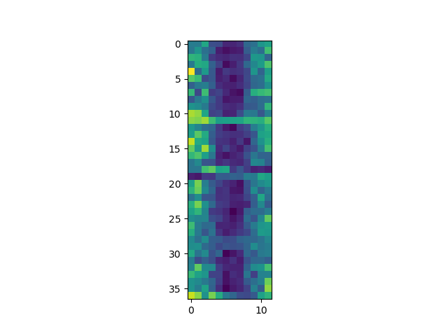
Each row in the heat map corresponds to a year in the dataset, and each column corresponds to a month. Blue pixels in this heat map represent low values, while yellow pixels represent high values. We can see low blue values in the middle (summer) months, and higher waves at the start and end of the year. This demonstrates that there is a seasonal cycle present. With calm summers bringing lower waves, and windy winters generating big waves. There are still differences year to year, with some stormier summers and calmer winters.

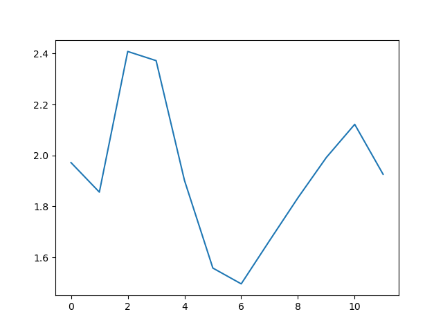
Now let’s take a look at the average wave-height per month over time:

ave_waveheight = numpy.mean(data, axis=0)
ave_plot = matplotlib.pyplot.plot(ave_waveheight)
matplotlib.pyplot.show()

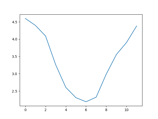
This is a good way to smooth out variability, and see what is called a ‘climatology’, representing the long-term wave climate over several years or decades.

Here, we have put the average wave heights per month across all years in the data ave_waveheight, then asked matplotlib.pyplot to create and display a line graph of those values. The result is a smooth seasonal cycle, with a maximum in month 0 (January) and minimum in month 6 (July). But a good data scientist doesn’t just consider the average of a dataset, so let’s have a look at two other statistics:

max_plot = matplotlib.pyplot.plot(numpy.max(data, axis=0))
matplotlib.pyplot.show()

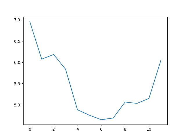
min_plot = matplotlib.pyplot.plot(numpy.min(data, axis=0))
matplotlib.pyplot.show()

The minimum and maximum graphs show the large spread of all possible wave heights throughout the dataset. There is still a seasonal cycle, but less clear as the extremes are much less smooth. The maximum wave heights can reach a massive 7 metres, and even in the summer the maximum is 4.5m (around the height of a double decker bus!) The minimum values are more similar throughout the year, varying between 1.5 and 2.5 metres.

Plotting the data in this way, allows us to get a broad picture of the wave climate, without having to examine the numbers themselves without visualization tools.

Grouping plots

You can group similar plots in a single figure using subplots. This script below uses a number of new commands. The function matplotlib.pyplot.figure() creates a space into which we will place all of our plots. The parameter figsize tells Python how big to make this space. Each subplot is placed into the figure using its add_subplot method. The add_subplot method takes 3 parameters. The first denotes how many total rows of subplots there are, the second parameter refers to the total number of subplot columns, and the final parameter denotes which subplot your variable is referencing (left-to-right, top-to-bottom). Each subplot is stored in a different variable (axes1, axes2, axes3). Once a subplot is created, the axes can be titled using the set_xlabel() command (or set_ylabel()). Let’s create three new plots, side by side, this time showing within each of the 37 years of the dataset - notice how we now use axis=1 in our calls to the summary statistic functions:

fig = matplotlib.pyplot.figure(figsize=(10.0, 3.0))

axes1 = fig.add_subplot(1, 3, 1)
axes2 = fig.add_subplot(1, 3, 2)
axes3 = fig.add_subplot(1, 3, 3)

axes1.set_ylabel('Average')
axes1.set_xlabel('Year index')
axes1.plot(numpy.mean(data, axis=1))

axes2.set_ylabel('Max')
axes2.set_xlabel('Year index')
axes2.plot(numpy.max(data, axis=1))

axes3.set_ylabel('Min')
axes3.set_xlabel('Year index')
axes3.plot(numpy.min(data, axis=1))

fig.tight_layout()

matplotlib.pyplot.savefig('wavedata.png')
matplotlib.pyplot.show()

This script tells the plotting library how large we want the figure to be, that we’re creating three subplots, what to draw for each one, and that we want a tight layout. (If we leave out that call to fig.tight_layout(), the graphs will actually be squeezed together more closely.)

The call to savefig stores the plot as a graphics file. This can be a convenient way to store your plots for use in other documents, web pages etc. The graphics format is automatically determined by Matplotlib from the file name ending we specify; here PNG from ‘wavedata.png’. Matplotlib supports many different graphics formats, including SVG, PDF, and JPEG.

Importing libraries with shortcuts

In this lesson we use the import matplotlib.pyplot syntax to import the pyplot module of matplotlib. However, shortcuts such as import matplotlib.pyplot as plt are frequently used. Importing pyplot this way means that after the initial import, rather than writing matplotlib.pyplot.plot(...), you can now write plt.plot(...). Another common convention is to use the shortcut import numpy as np when importing the NumPy library. We then can write np.loadtxt(...) instead of numpy.loadtxt(...), for example.

Some people prefer these shortcuts as it is quicker to type and results in shorter lines of code - especially for libraries with long names! You will frequently see Python code online using a pyplot function with plt, or a NumPy function with np, and it’s because they’ve used this shortcut. It makes no difference which approach you choose to take, but you must be consistent as if you use import matplotlib.pyplot as plt then matplotlib.pyplot.plot(...) will not work, and you must use plt.plot(...) instead. Because of this, when working with other people it is important you agree on how libraries are imported.

Plot Scaling

Why do all of our plots stop just short of the upper end of our graph?

Solution

Because matplotlib normally sets x and y axes limits to the min and max of our data (depending on data range)

If we want to change this, we can use the set_ylim(min, max) method of each ‘axes’, for example:

axes3.set_ylim(0,8)

Update your plotting code to automatically set a more appropriate scale. (Hint: you can make use of the max and min methods to help.)

Solution

# One method
axes3.set_ylabel('min')
axes3.plot(numpy.min(data, axis=1))
axes3.set_ylim(0,8)

Solution

# A more automated approach
min_data = numpy.min(data, axis=1)
axes3.set_ylabel('min')
axes3.plot(min_data)
axes3.set_ylim(numpy.nanmin(min_data), numpy.nanmax(min_data) * 1.1)

Plotting multiple graphs on one pair of axes

We can also plot more than one dataset on a single pair of axes, and Matplotlib gives us lots of control over the output. Can you plot the maximum, minimum, and mean all on the same axes, change the colour and marker used for each of the plots, and give the plot a legend?

Solution

We can call plot multiple times before we call show, and each of those will be added to the axes. We can also specify format options as a string (this needs to specified straight after the data to plot), with all available options listed in the documentation. We also need to specify labels for each plot, and call legend() to make the legend visible.

An example would be

matplotlib.pyplot.plot(numpy.max(data, axis=0), "bo", label='Maximum')
matplotlib.pyplot.plot(numpy.average(data, axis=0), "m+", label='Average')
matplotlib.pyplot.plot(numpy.min(data, axis=0), "r--", label='Minumum')
matplotlib.pyplot.legend(loc='best')

matplotlib.pyplot.show()

Make Your Own Plot

Create a plot showing the standard deviation (numpy.std) of the wave data across all months.

Solution

std_plot = matplotlib.pyplot.plot(numpy.std(data, axis=0))
matplotlib.pyplot.show()

Moving Plots Around

Modify the program to display the three plots on top of one another instead of side by side.

Solution

# change figsize (swap width and height)
fig = matplotlib.pyplot.figure(figsize=(3.0, 10.0))

# change add_subplot (swap first two parameters)
axes1 = fig.add_subplot(3, 1, 1)
axes2 = fig.add_subplot(3, 1, 2)
axes3 = fig.add_subplot(3, 1, 3)

axes1.set_ylabel('average')
axes1.plot(numpy.mean(data, axis=1))

axes2.set_ylabel('max')
axes2.plot(numpy.max(data, axis=1))

axes3.set_ylabel('min')
axes3.plot(numpy.min(data, axis=1))

fig.tight_layout()

matplotlib.pyplot.show()

Key Points

• Use the pyplot module from the matplotlib library for creating simple visualizations.

Storing Multiple Values in Lists

Overview

Teaching: 30 min
Exercises: 15 min

Questions

• How can I store many values together?

Objectives

• Explain what a list is.

• Create and index lists of simple values.

• Change the values of individual elements

• Append values to an existing list

• Reorder and slice list elements

• Create and manipulate nested lists

In the previous episode, we analyzed a single file of wave height data. Let’s now look at analysing multiple files, for example to look at data over a set of different regions or times.

The natural first step is to collect the names of all the files that we have to process. In Python, a list is a way to store multiple values together. In this episode, we will learn how to store multiple values in a list as well as how to work with lists.

Python lists

Unlike NumPy arrays, lists are built into the language so we do not have to load a library to use them. We create a list by putting values inside square brackets and separating the values with commas:

odds = [1, 3, 5, 7]
print('odds are:', odds)

odds are: [1, 3, 5, 7]

We can access elements of a list using indices – numbered positions of elements in the list. These positions are numbered starting at 0, so the first element has an index of 0.

print('first element:', odds[0])
print('last element:', odds[3])
print('"-1" element:', odds[-1])

first element: 1
last element: 7
"-1" element: 7

Yes, we can use negative numbers as indices in Python. When we do so, the index -1 gives us the last element in the list, -2 the second to last, and so on. Because of this, odds[3] and odds[-1] point to the same element here.

There is one important difference between lists and strings: we can change the values in a list, but we cannot change individual characters in a string. For example:

names = ['Curie', 'Darwing', 'Turing']  # typo in Darwin's name
print('names is originally:', names)
names[1] = 'Darwin'  # correct the name
print('final value of names:', names)

names is originally: ['Curie', 'Darwing', 'Turing']
final value of names: ['Curie', 'Darwin', 'Turing']

works, but:

name = 'Darwin'
name[0] = 'd'

---------------------------------------------------------------------------
TypeError                                 Traceback (most recent call last)
<ipython-input-8-220df48aeb2e> in <module>()
      1 name = 'Darwin'
----> 2 name[0] = 'd'

TypeError: 'str' object does not support item assignment

does not.

Ch-Ch-Ch-Ch-Changes

Data which can be modified in place is called mutable, while data which cannot be modified is called immutable. Strings and numbers are immutable. This does not mean that variables with string or number values are constants, but when we want to change the value of a string or number variable, we can only replace the old value with a completely new value.

Lists and arrays, on the other hand, are mutable: we can modify them after they have been created. We can change individual elements, append new elements, or reorder the whole list. For some operations, like sorting, we can choose whether to use a function that modifies the data in-place or a function that returns a modified copy and leaves the original unchanged.

Be careful when modifying data in-place. If two variables refer to the same list, and you modify the list value, it will change for both variables!

salsa = ['peppers', 'onions', 'coriander', 'tomatoes']
my_salsa = salsa        # <-- my_salsa and salsa point to the *same* list data in memory
salsa[0] = 'hot peppers'
print('Ingredients in my salsa:', my_salsa)

Ingredients in my salsa: ['hot peppers', 'onions', 'coriander', 'tomatoes']

If you want variables with mutable values to be independent, you must make a copy of the value when you assign it.

salsa = ['peppers', 'onions', 'coriander', 'tomatoes']
my_salsa = list(salsa)        # <-- makes a *copy* of the list
salsa[0] = 'hot peppers'
print('Ingredients in my salsa:', my_salsa)

Ingredients in my salsa: ['peppers', 'onions', 'coriander', 'tomatoes']

Because of pitfalls like this, code which modifies data in place can be more difficult to understand. However, it is often far more efficient to modify a large data structure in place than to create a modified copy for every small change. You should consider both of these aspects when writing your code.

Nested Lists

Since a list can contain any Python variables, it can even contain other lists.

For example, we could represent the products in the shelves of a small grocery shop:

x = [['pepper', 'courgette', 'onion'],
     ['cabbage', 'lettuce', 'garlic'],
     ['apple', 'pear', 'banana']]

Here is a visual example of how indexing a list of lists x works:

Using the previously declared list x, these would be the results of the index operations shown in the image:

print([x[0]])

[['pepper', 'courgette', 'onion']]

print(x[0])

['pepper', 'courgette', 'onion']

print(x[0][0])

'pepper'

Thanks to Hadley Wickham for the image above.

Heterogeneous Lists

Lists in Python can contain elements of different types. Example:

sample_ages = [10, 12.5, 'Unknown']

There are many ways to change the contents of lists besides assigning new values to individual elements:

odds.append(11)
print('odds after adding a value:', odds)

odds after adding a value: [1, 3, 5, 7, 11]

removed_element = odds.pop(0)
print('odds after removing the first element:', odds)
print('removed_element:', removed_element)

odds after removing the first element: [3, 5, 7, 11]
removed_element: 1

odds.reverse()
print('odds after reversing:', odds)

odds after reversing: [11, 7, 5, 3]

While modifying in place, it is useful to remember that Python treats lists in a slightly counter-intuitive way.

As we saw earlier, when we modified the salsa list item in-place, if we make a list, (attempt to) copy it and then modify this list, we can cause all sorts of trouble. This also applies to modifying the list using the above functions:

odds = [3, 5, 7]
primes = odds
primes.append(2)
print('primes:', primes)
print('odds:', odds)

primes: [3, 5, 7, 2]
odds: [3, 5, 7, 2]

This is because Python stores a list in memory, and then can use multiple names to refer to the same list. If all we want to do is copy a (simple) list, we can again use the list function, so we do not modify a list we did not mean to:

odds = [3, 5, 7]
primes = list(odds)
primes.append(2)
print('primes:', primes)
print('odds:', odds)

primes: [3, 5, 7, 2]
odds: [3, 5, 7]

Subsets of lists and strings can be accessed by specifying ranges of values in brackets, similar to how we accessed ranges of positions in a NumPy array. This is commonly referred to as “slicing” the list/string.

binomial_name = 'Drosophila melanogaster'
group = binomial_name[0:10]
print('group:', group)

species = binomial_name[11:23]
print('species:', species)

chromosomes = ['X', 'Y', '2', '3', '4']
autosomes = chromosomes[2:5]
print('autosomes:', autosomes)

last = chromosomes[-1]
print('last:', last)

group: Drosophila
species: melanogaster
autosomes: ['2', '3', '4']
last: 4

Slicing From the End

Use slicing to access only the last four characters of a string or entries of a list.

string_for_slicing = 'Observation date: 02-Feb-2013'
list_for_slicing = [['fluorine', 'F'],
                    ['chlorine', 'Cl'],
                    ['bromine', 'Br'],
                    ['iodine', 'I'],
                    ['astatine', 'At']]

'2013'
[['chlorine', 'Cl'], ['bromine', 'Br'], ['iodine', 'I'], ['astatine', 'At']]

Would your solution work regardless of whether you knew beforehand the length of the string or list (e.g. if you wanted to apply the solution to a set of lists of different lengths)? If not, try to change your approach to make it more robust.

Hint: Remember that indices can be negative as well as positive

Solution

Use negative indices to count elements from the end of a container (such as list or string):

string_for_slicing[-4:]
list_for_slicing[-4:]

Non-Continuous Slices

So far we’ve seen how to use slicing to take single blocks of successive entries from a sequence. But what if we want to take a subset of entries that aren’t next to each other in the sequence?

You can achieve this by providing a third argument to the range within the brackets, called the step size. The example below shows how you can take every third entry in a list:

primes = [2, 3, 5, 7, 11, 13, 17, 19, 23, 29, 31, 37]
subset = primes[0:12:3]
print('subset', subset)

subset [2, 7, 17, 29]

Notice that the slice taken begins with the first entry in the range, followed by entries taken at equally-spaced intervals (the steps) thereafter. If you wanted to begin the subset with the third entry, you would need to specify that as the starting point of the sliced range:

primes = [2, 3, 5, 7, 11, 13, 17, 19, 23, 29, 31, 37]
subset = primes[2:12:3]
print('subset', subset)

subset [5, 13, 23, 37]

Use the step size argument to create a new string that contains only every other character in the string “In an octopus’s garden in the shade”. Start with creating a variable to hold the string:

beatles = "In an octopus's garden in the shade"

What slice of beatles will produce the following output (i.e., the first character, third character, and every other character through the end of the string)?

I notpssgre ntesae

Solution

To obtain every other character you need to provide a slice with the step size of 2:

beatles[0:35:2]

You can also leave out the beginning and end of the slice to take the whole string and provide only the step argument to go every second element:

beatles[::2]

If you want to take a slice from the beginning of a sequence, you can omit the first index in the range:

date = 'Monday 4 January 2016'
day = date[0:6]
print('Using 0 to begin range:', day)
day = date[:6]
print('Omitting beginning index:', day)

Using 0 to begin range: Monday
Omitting beginning index: Monday

And similarly, you can omit the ending index in the range to take a slice to the very end of the sequence:

months = ['jan', 'feb', 'mar', 'apr', 'may', 'jun', 'jul', 'aug', 'sep', 'oct', 'nov', 'dec']
sond = months[8:12]
print('With known last position:', sond)
sond = months[8:len(months)]
print('Using len() to get last entry:', sond)
sond = months[8:]
print('Omitting ending index:', sond)

With known last position: ['sep', 'oct', 'nov', 'dec']
Using len() to get last entry: ['sep', 'oct', 'nov', 'dec']
Omitting ending index: ['sep', 'oct', 'nov', 'dec']

Overloading

+ usually means addition, but when used on strings or lists, it means “concatenate”. Given that, what do you think the multiplication operator * does on lists? In particular, what will be the output of the following code?

counts = [2, 4, 6, 8, 10]
repeats = counts * 2
print(repeats)

1. [2, 4, 6, 8, 10, 2, 4, 6, 8, 10]
2. [4, 8, 12, 16, 20]
3. [[2, 4, 6, 8, 10],[2, 4, 6, 8, 10]]
4. [2, 4, 6, 8, 10, 4, 8, 12, 16, 20]

The technical term for this is operator overloading: a single operator, like + or *, can do different things depending on what it’s applied to.

Solution

The multiplication operator * used on a list replicates elements of the list and concatenates them together:

[2, 4, 6, 8, 10, 2, 4, 6, 8, 10]

It’s equivalent to:

counts + counts

This behaviour is specific to lists - if we were to do the same thing in a NumPy array, we would get something like:

counts = nump.array([2, 4, 6, 8, 10])
repeats = counts * 2
print(repeats)

`[4, 8, 12, 16, 20]`

Key Points

• [value1, value2, value3, ...] creates a list.

• Lists can contain any Python object, including lists (i.e., list of lists).

• Lists are indexed and sliced with square brackets (e.g., list[0] and list[2:9]), in the same way as strings and arrays.

• Lists are mutable (i.e., their values can be changed in place).

• Strings are immutable (i.e., the characters in them cannot be changed).

Repeating Actions with Loops

Overview

Teaching: 30 min
Exercises: 0 min

Questions

• How can I do the same operations on many different values?

Objectives

• Explain what a for loop does.

• Correctly write for loops to repeat simple calculations.

• Trace changes to a loop variable as the loop runs.

• Trace changes to other variables as they are updated by a for loop.

In the episode about visualizing data, we wrote Python code that plots values of interest from the wave-height dataset. What would happen if we want to create plots for all more data sets with a single statement. To do that, we’ll have to teach the computer how to repeat things.

An example task that we might want to repeat is accessing numbers in a list, which we will do by printing each number on a line of its own.

odds = [1, 3, 5, 7]

In Python, a list is basically an ordered collection of elements, and every element has a unique number associated with it — its index. This means that we can access elements in a list using their indices. For example, we can get the first number in the list odds, by using odds[0]. One way to print each number is to use four print statements:

print(odds[0])
print(odds[1])
print(odds[2])
print(odds[3])

1
3
5
7

This is a bad approach for three reasons:

1. Not scalable. Imagine you need to print a list that has hundreds of elements. It might be easier to type them in manually.

2. Difficult to maintain. If we want to decorate each printed element with an asterisk or any other character, we would have to change four lines of code. While this might not be a problem for small lists, it would definitely be a problem for longer ones.

3. Fragile. If we use it with a list that has more elements than what we initially envisioned, it will only display part of the list’s elements. A shorter list, on the other hand, will cause an error because it will be trying to display elements of the list that do not exist.

odds = [1, 3, 5]
print(odds[0])
print(odds[1])
print(odds[2])
print(odds[3])

1
3
5

---------------------------------------------------------------------------
IndexError                                Traceback (most recent call last)
<ipython-input-3-7974b6cdaf14> in <module>()
      3 print(odds[1])
      4 print(odds[2])
----> 5 print(odds[3])

IndexError: list index out of range

Here’s a better approach: a for loop

odds = [1, 3, 5, 7]
for num in odds:
    print(num)

1
3
5
7

This is shorter — certainly shorter than something that prints every number in a hundred-number list — and more robust as well:

odds = [1, 3, 5, 7, 9, 11]
for num in odds:
    print(num)

1
3
5
7
9
11

The improved version uses a for loop to repeat an operation — in this case, printing — once for each thing in a sequence. The general form of a loop is:

for variable in collection:
    # do things using variable, such as print

Using the odds example above, the loop might look like this:

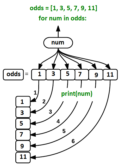
where each number (num) in the variable odds is looped through and printed one number after another. The other numbers in the diagram denote which loop cycle the number was printed in (1 being the first loop cycle, and 6 being the final loop cycle).

We can call the loop variable anything we like, but there must be a colon at the end of the line starting the loop, and we must indent anything we want to run inside the loop. Unlike many other languages, there is no command to signify the end of the loop body (e.g. end for); what is indented after the for statement belongs to the loop.

What’s in a name?

In the example above, the loop variable was given the name num as a mnemonic; it is short for ‘number’. We can choose any name we want for variables. We might just as easily have chosen the name banana for the loop variable, as long as we use the same name when we invoke the variable inside the loop:

odds = [1, 3, 5, 7, 9, 11]
for banana in odds:
    print(banana)

1
3
5
7
9
11

It is a good idea to choose variable names that are meaningful, otherwise it would be more difficult to understand what the loop is doing.

Here’s another loop that repeatedly updates a variable:

length = 0
names = ['Curie', 'Darwin', 'Turing']
for value in names:
    length = length + 1
print('There are', length, 'names in the list.')

There are 3 names in the list.

It’s worth tracing the execution of this little program step by step. Since there are three names in names, the statement on line 4 will be executed three times. The first time around, length is zero (the value assigned to it on line 1) and value is Curie. The statement adds 1 to the old value of length, producing 1, and updates length to refer to that new value. The next time around, value is Darwin and length is 1, so length is updated to be 2. After one more update, length is 3; since there is nothing left in names for Python to process, the loop finishes and the print function on line 5 tells us our final answer.

Note that a loop variable is a variable that is being used to record progress in a loop. It still exists after the loop is over, and we can re-use variables previously defined as loop variables as well:

name = 'Rosalind'
for name in ['Curie', 'Darwin', 'Turing']:
    print(name)
print('after the loop, name is', name)

Curie
Darwin
Turing
after the loop, name is Turing

Note also that finding the length of an object is such a common operation that Python actually has a built-in function to do it called len:

print(len([0, 1, 2, 3]))

4

len is much faster than any function we could write ourselves, and much easier to read than a two-line loop; it will also give us the length of many other things that we haven’t met yet, so we should always use it when we can.

From 1 to N

Python has a built-in function called range that generates a sequence of numbers. range can accept 1, 2, or 3 parameters.

• If one parameter is given, range generates a sequence of that length, starting at zero and incrementing by 1. For example, range(3) produces the numbers 0, 1, 2.
• If two parameters are given, range starts at the first and ends just before the second, incrementing by one. For example, range(2, 5) produces 2, 3, 4.
• If range is given 3 parameters, it starts at the first one, ends just before the second one, and increments by the third one. For example, range(3, 10, 2) produces 3, 5, 7, 9.

Using range, write a loop that uses range to print the first 3 natural numbers:

1
2
3

Solution

for number in range(1, 4):
    print(number)

Understanding the loops

Given the following loop:

word = 'oxygen'
for char in word:
    print(char)

How many times is the body of the loop executed?

• 3 times
• 4 times
• 5 times
• 6 times

Solution

The body of the loop is executed 6 times.

Computing Powers With Loops

Exponentiation is built into Python:

print(5 ** 3)

125

Write a loop that calculates the same result as 5 ** 3 using multiplication (and without exponentiation).

Solution

result = 1
for number in range(0, 3):
    result = result * 5
print(result)

Summing a list

Write a loop that calculates the sum of elements in a list by adding each element and printing the final value, so [124, 402, 36] prints 562

Solution

numbers = [124, 402, 36]
summed = 0
for num in numbers:
    summed = summed + num
print(summed)

Computing the Value of a Polynomial

The built-in function enumerate takes a sequence (e.g. a list) and generates a new sequence of the same length. Each element of the new sequence is a pair composed of the index (0, 1, 2,…) and the value from the original sequence:

for idx, val in enumerate(a_list):
    # Do something using idx and val

The code above loops through a_list, assigning the index to idx and the value to val.

Suppose you have encoded a polynomial as a list of coefficients in the following way: the first element is the constant term, the second element is the coefficient of the linear term, the third is the coefficient of the quadratic term, etc.

x = 5
coefs = [2, 4, 3]
y = coefs[0] * x**0 + coefs[1] * x**1 + coefs[2] * x**2
print(y)

97

Write a loop using enumerate(coefs) which computes the value y of any polynomial, given x and coefs.

Solution

y = 0
for idx, coef in enumerate(coefs):
    y = y + coef * x**idx

Key Points

• Use for variable in sequence to process the elements of a sequence one at a time.

• The body of a for loop must be indented.

• Use len(thing) to determine the length of something that contains other values.

Analyzing Data from Multiple Files

Overview

Teaching: 20 min
Exercises: 0 min

Questions

• How can I do the same operations on many different files?

Objectives

• Use a library function to get a list of filenames that match a wildcard pattern.

• Write a for loop to process multiple files.

When working with real datasets, we may not always have everything in a single file. We need a way to get a list of all the files in our data directory whose names start with wave- and end with .csv. The following library will help us to achieve this:

import glob

The glob library contains a function, also called glob, that finds files and directories whose names match a pattern. We provide those patterns as strings: the character * matches zero or more characters, while ? matches any one character. We can use this to get the names of all the CSV files in the current directory:

print(glob.glob('waves_*.csv'))

['waves_10s.csv', 'waves_00s.csv', 'waves_80s.csv', 'waves_90s.csv']

These files show waveheight data from some years in the decades indicated in the filename. As these examples show, glob.glob’s result is a list of file and directory paths in arbitrary order. This means we can loop over it to do something with each filename in turn. In our case, the “something” we want to do is generate a set of plots for each file in our waveheight dataset.

If we want to start by analyzing just the first three files in alphabetical order, we can use the sorted built-in function to generate a new sorted list from the glob.glob output:

import glob
import numpy
import matplotlib.pyplot

filenames = sorted(glob.glob('waves_*.csv'))
filenames = filenames[0:3]

for filename in filenames:
    print(filename)
    
    data = numpy.loadtxt(fname=filename, delimiter=',')
    number_of_rows = data.shape[0]
    number_of_years = number_of_rows//12

    # need to reshape the data for plotting
    data = numpy.reshape(data[:,2], [number_of_years,12])
    
    fig = matplotlib.pyplot.figure(figsize=(10.0, 3.0))
        
    axes1 = fig.add_subplot(1, 3, 1)
    axes2 = fig.add_subplot(1, 3, 2)
    axes3 = fig.add_subplot(1, 3, 3)

    axes1.set_ylabel('average')
    axes1.plot(numpy.mean(data, axis=0))

    axes2.set_ylabel('max')
    axes2.plot(numpy.max(data, axis=0))

    axes3.set_ylabel('min')
    axes3.plot(numpy.min(data, axis=0))

    fig.tight_layout()
    matplotlib.pyplot.show()

waves-00.csv

waves-10s.csv

waves-80s.csv

Looking at these three decades, we can see similarities - with the average value representing a smooth climate with clear annual cycle. There are differences year on year, and the minimum and maximum data tend to be more variable than the mean.

Different types of division

You might have noticed that we calculated the number of years when reshaping the data, rather than using 10 for each decade. This was useful here because the file containing data from the 2010s only has data from 6 years, but each one of these years did contain data for every month. If any year had missing data from any month, we would have needed to have done some additional preprocessing.

When we divided by 12 to get the number of years, we used // - you might have expected us just to use /. Python creates a float as a result from a division operation using /, even if both inputs are integers:

type(10/2)

float

However, if you use a float value as an array index, you get an error (even if it refers to a whole number). // is Python’s integer division operator - meaning that the result will always be an integer:

type(10//2)

int

If the result would normally result in a floating-point number, the actual result will instead be an integer rounded towards minus infinity:

print(19/4)
print(19//4)

4.75
4

Sometimes, plots can help us spot patterns in data, or problems with data.

Let’s load waves_90s.csv:

data = numpy.loadtxt(fname = "waves_90s.csv", delimiter=',')

If we try and take the mean for the entire year, we’ll see that there must be NaNs:

numpy.mean(data[:,2])

nan

If we had only plotted the reshaped data, we would see white squares where there are NaNs in the data:

matplotlib.pyplot.imshow(data)
matplotlib.pyplot.show()

We can clearly see that there must have been some problem with the collection of data in the first 6 months of 1994. Apart from that, the rest of the data looks relatively sensible, with low wave heights in the summer months of the decade, and higher wave heights in the winter months of the decade. This means that we have no reason not to trust the rest of the dataset.

There are other ways that we could have determined where the missing data is. The Numpy function isnan will tell us whether any given value is NaN; if we give it an ndarray, it will return an ndarray of the same shape with boolean values (True or False) showing if the value at that index was a NaN. argwhere will return the indices for an ndarray of booleans where the value is True.

numpy.argwhere(numpy.isnan(data))

array([[4, 0],
       [4, 1],
       [4, 2],
       [4, 3],
       [4, 4],
       [4, 5]])

There are almost always multiple ways to achieve the same result in programming, and often the choice as to which method to use comes down to personal preference. Some people might prefer to look at patterns in plots, while others may be happy to look at summary statistics and aggregate values from tabular data to come to the same conclusion.

Plotting Differences

Plot the difference between the average monthly waveheights in the 1980s and 1990s Can you do this using glob, without specifying the filenames explicitly in the code?

Solution

import glob
import numpy
import matplotlib.pyplot

filenames = sorted(glob.glob('waves_*.csv'))

data0 = numpy.loadtxt(fname=filenames[2], delimiter=',')
data1 = numpy.loadtxt(fname=filenames[3], delimiter=',')

number_of_rows0 = data0.shape[0]
number_of_years0 = number_of_rows0//12 
data0 = numpy.reshape(data0[:,2], [number_of_years0,12])

number_of_rows1 = data1.shape[0]
number_of_years1 = number_of_rows1//12 
data1 = numpy.reshape(data1[:,2], [number_of_years1,12])

fig = matplotlib.pyplot.figure(figsize=(10.0, 3.0))

matplotlib.pyplot.ylabel('Difference in average')
matplotlib.pyplot.plot(numpy.mean(data0, axis=0) - numpy.mean(data1, axis=0))

fig.tight_layout()
matplotlib.pyplot.show()

Congratulations! We’ve investigated the wave data and spotted some trends, and identified bad / missing data. Now that we understand what is in the model data set, and trust that it is realistic, we can use it to make practical decisions about things like boat operations!

Key Points

• Use glob.glob(pattern) to create a list of files whose names match a pattern.

• Use * in a pattern to match zero or more characters, and ? to match any single character.

Making Choices

Overview

Teaching: 30 min
Exercises: 0 min

Questions

• How can my programs do different things based on data values?

Objectives

• Write conditional statements including if, elif, and else branches.

• Correctly evaluate expressions containing and and or.

In our previous lessons, we examined the seasonal behaviour of sea waves. How can we use this data to make practical decisions?

How can we use Python to identify thresholds, and take a different action for each? In this lesson, we’ll learn how to write code that runs only when certain conditions are true.

Conditionals

We can ask Python to take different actions, depending on a condition, with an if statement:

num = 37
if num > 100:
    print('greater')
else:
    print('not greater')
print('done')

not greater
done

The second line of this code uses the keyword if to tell Python that we want to make a choice. If the test that follows the if statement is true, the body of the if (i.e., the set of lines indented underneath it) is executed, and “greater” is printed. If the test is false, the body of the else is executed instead, and “not greater” is printed. Only one or the other is ever executed before continuing on with program execution to print “done”:

Conditional statements don’t have to include an else. If there isn’t one, Python simply does nothing if the test is false:

num = 53
print('before conditional...')
if num > 100:
    print(num, 'is greater than 100')
print('...after conditional')

before conditional...
...after conditional

We can also chain several tests together using elif, which is short for “else if”. The following Python code uses elif to print the sign of a number.

num = -3

if num > 0:
    print(num, 'is positive')
elif num == 0:
    print(num, 'is zero')
else:
    print(num, 'is negative')

-3 is negative

Note that to test for equality we use a double equals sign == rather than a single equals sign = which is used to assign values.

Comparing in Python

Along with the > and == operators we have already used for comparing values in our conditionals, there are a few more options to know about:

• >: greater than
• <: less than
• ==: equal to
• !=: does not equal
• >=: greater than or equal to
• <=: less than or equal to

We can also combine tests using and and or. and is only true if both parts are true:

if (1 > 0) and (-1 >= 0):
    print('both parts are true')
else:
    print('at least one part is false')

at least one part is false

while or is true if at least one part is true:

if (1 < 0) or (1 >= 0):
    print('at least one test is true')

at least one test is true

True and False

True and False are special words in Python called booleans, which represent truth values. A statement such as 1 < 0 returns the value False, while -1 < 0 returns the value True.

Checking our Data

Now that we’ve seen how conditionals work, we can use them to look for thresholds in our wave data. We are about to use functions provided by the numpy module again. Therefore, if you’re working in a new Python session, make sure to load the module with:

import numpy

If you are operating a boat, for carrying passengers of working offshore, you need to know that it will be save to go to sea. Ideally you wouldn’t want to have passengers transported if the wave height is above 3 metres.

Let’s look at our wave data, and find which months we can operate the boats, based on the monthly mean wave-height.

We could look at each month individually:

month0 = numpy.mean(data, axis=0)[0] # [0] gets the first element of the array. In our case, the first month: January

if month0 < 3:
    print('Can take passengers this month')

Survey vehicles can operate in stormier waters, with wave heights up to 4m

elif numpy.mean(data, axis=0) < 4:
    print('Can take survey vehicles (but not passengers)')

And if neither of these conditions are true, then it’s too stormy, and nothing can go out.

else:
    print('Can't take any boats out to sea')

Let’s test that out for January:

data = numpy.loadtxt(fname='reshaped_data.csv', delimiter=',')

month0 = numpy.mean(data, axis=0)[0]

if month0 < 3:
    print('Can take passengers this month')
elif numpy.mean(data, axis=0) < 4:
    print('Can take survey vehicles (but not passengers)')
else:
    print('Can't take any boats out to sea')

Can't take any boats out to sea

Now let’s try for June

month5 = numpy.mean(data, axis=0)[5]

if month5 < 3:
    print('Can take passengers this month')
elif numpy.mean(data, axis=0) < 4:
    print('Can take survey vehicles (but not passengers)')
else:
    print('Can't take any boats out to sea')

Can take passengers this month

Notice how the statement stops as soon as it reaches a condition which is True.

We could test for all months less manually, using a for loop:

for month_index, monthly_waveheight in enumerate(numpy.mean(r, axis=0)):
    if monthly_waveheight < 3:
        print(f"Month {month_index}: we can take passengers this month")
    elif monthly_waveheight < 4:
        print(f"Month {month_index}: we can take survey vehicles (but not passengers) this month")
    else:
        print(f"Month {month_index}: we can't take any boats out to sea this month")

Month 0: can't take any boats out to sea this month
Month 1: can't take any boats out to sea this month
Month 2: can't take any boats out to sea this month
Month 3: can take survey vehicles (but not passengers) this month
Month 4: can take passengers this month
Month 5: can take passengers this month
Month 6: can take passengers this month
Month 7: can take passengers this month
Month 8: can take passengers this month
Month 9: can take survey vehicles (but not passengers) this month
Month 10: can take survey vehicles (but not passengers) this month
Month 11: can't take any boats out to sea this month

The enumerate function is the Pythonic way of getting the index of values in a loop - in this case it allows us to list the month number in the output. We need a variable to store this value in, which we’re calling month_index. Because the loop returns two variables form each iteration (month index and monthly waveheight), we need two variables.

We can see that we could suggest a timetable for passenger ferries in May - September (inclusive), we could plan to take survey boats out in April, October, and November; and we should not plan any sea-going activities in January, February, March, or December.

This is a relatively crude example, but shows how we can use these programming constructs to help make some decisions using the data.

In this way, we have asked Python to do something different depending on the condition of our data. Here we printed messages in all cases, but we could also imagine not using the else catch-all so that messages are only printed when something is wrong, freeing us from having to manually examine every plot for features we’ve seen before.

How Many Paths?

Consider this code:

if 4 > 5:
    print('A')
elif 4 == 5:
    print('B')
elif 4 < 5:
    print('C')

Which of the following would be printed if you were to run this code? Why did you pick this answer?

1. A
2. B
3. C
4. B and C

Solution

C gets printed because the first two conditions, 4 > 5 and 4 == 5, are not true, but 4 < 5 is true.

What Is Truth?

True and False booleans are not the only values in Python that are true and false. In fact, any value can be used in an if or elif. After reading and running the code below, explain what the rule is for which values are considered true and which are considered false.

if '':
    print('empty string is true')
if 'word':
    print('word is true')
if []:
    print('empty list is true')
if [1, 2, 3]:
    print('non-empty list is true')
if 0:
    print('zero is true')
if 1:
    print('one is true')

That’s Not Not What I Meant

Sometimes it is useful to check whether some condition is not true. The Boolean operator not can do this explicitly. After reading and running the code below, write some if statements that use not to test the rule that you formulated in the previous challenge.

if not '':
    print('empty string is not true')
if not 'word':
    print('word is not true')
if not not True:
    print('not not True is true')

Close Enough

Write some conditions that print True if the variable a is within 10% of the variable b and False otherwise. Compare your implementation with your partner’s: do you get the same answer for all possible pairs of numbers?

Hint

There is a built-in function abs that returns the absolute value of a number:

print(abs(-12))

12

Solution 1

a = 5
b = 5.1

if abs(a - b) <= 0.1 * abs(b):
    print('True')
else:
    print('False')

Solution 2

print(abs(a - b) <= 0.1 * abs(b))

This works because the Booleans True and False have string representations which can be printed.

In-Place Operators

Python (and most other languages in the C family) provides in-place operators that work like this:

x = 1  # original value
x += 1 # add one to x, assigning result back to x
x *= 3 # multiply x by 3
print(x)

6

Write some code that sums the positive and negative numbers in a list separately, using in-place operators. Do you think the result is more or less readable than writing the same without in-place operators?

Solution

positive_sum = 0
negative_sum = 0
test_list = [3, 4, 6, 1, -1, -5, 0, 7, -8]
for num in test_list:
    if num > 0:
        positive_sum += num
    elif num == 0:
        pass
    else:
        negative_sum += num
print(positive_sum, negative_sum)

Here pass means “don’t do anything”. In this particular case, it’s not actually needed, since if num == 0 neither sum needs to change, but it illustrates the use of elif and pass.

Sorting a List Into Buckets

In our data folder, we have some CSV files (those with .csv file extensions), and one NetCDF file (with a .nc file extension). We’d like to break these files into two lists called csv_files and nc_files, respectively.

Add code to the template below to do this. Note that the string method startswith returns True if and only if the string it is called on ends with the string passed as an argument, that is:

'String'.endswith('ing')

True

But

'String'.endswith('ING')

False

Use the following Python code as your starting point:

filenames = ['wavesmonthly.csv',
         'waves_00s.csv',
         'waves_10s.csv',
         'waves_80s.csv',
         'waves_90s.csv',
         'multyear_hs_avg.nc']
csv_files = []
nc_files = []

Your solution should:

1. loop over the names of the files
2. figure out which group each filename belongs in
3. append the filename to that list

In the end the two lists should be:

csv_files = ['waves_00s.csv', 'waves_10s.csv', 'waves_80s.csv', 'waves_90s.csv', 'wavesmonthly.csv']
nc_files = ['multyear_hs_avg.nc']

Solution

for filename in filenames:
    if filename.endswith('csv'):
        csv_files.append(filename)
    elif filename.endswith('nc'):
        nc_files.append(filename)
    else:
        other_files.append(filename)

print('csv_files:', csv_files)
print('nc_files:', nc_files)
print('other_files:', other_files)

Counting Vowels

1. Write a loop that counts the number of vowels in a character string.
2. Test it on a few individual words and full sentences.
3. Once you are done, compare your solution to your neighbor’s. Did you make the same decisions about how to handle the letter ‘y’ (which some people think is a vowel, and some do not)?

Solution

vowels = 'aeiouAEIOU'
sentence = 'Mary had a little lamb.'
count = 0
for char in sentence:
    if char in vowels:
        count += 1

print('The number of vowels in this string is ' + str(count))

Key Points

• Use if condition to start a conditional statement, elif condition to provide additional tests, and else to provide a default.

• The bodies of the branches of conditional statements must be indented.

• Use == to test for equality.

• X and Y is only true if both X and Y are true.

• X or Y is true if either X or Y, or both, are true.

• Zero, the empty string, and the empty list are considered false; all other numbers, strings, and lists are considered true.

• True and False represent truth values.