Creating Functions
Overview
Teaching: 30 min
Exercises: 0 minQuestions
How can I define new functions?
What’s the difference between defining and calling a function?
What happens when I call a function?
Objectives
Define a function that takes parameters.
Return a value from a function.
Test and debug a function.
Set default values for function parameters.
Explain why we should divide programs into small, single-purpose functions.
From yesterday we’ve seen that code can have Python make decisions about what it sees in our data. What if we want to convert some of our data, like taking a temperature in Fahrenheit and converting it to Celsius. We could write something like this for converting a single number
fahrenheit_val = 99
celsius_val = ((fahrenheit_val - 32) * (5/9))
and for a second number we could just copy the line and rename the variables
fahrenheit_val = 99
celsius_val = ((fahrenheit_val - 32) * (5/9))

fahrenheit_val2 = 43
celsius_val2 = ((fahrenheit_val2 - 32) * (5/9))
But we would be in trouble as soon as we had to do this more than a couple times.
Cutting and pasting it is going to make our code get very long and very repetitive,
very quickly.
We’d like a way to package our code so that it is easier to reuse,
a shorthand way of re-executing longer pieces of code. In Python we can use ‘functions’.
Let’s start by defining a function fahr_to_celsius that converts temperatures
from Fahrenheit to Celsius:
def explicit_fahr_to_celsius(temp):
    # Assign the converted value to a variable
    converted = ((temp - 32) * (5/9))
    # Return the value of the new variable
    return converted

def fahr_to_celsius(temp):
    # Return converted value more efficiently using the return
    # function without creating a new variable. This code does
    # the same thing as the previous function but it is more explicit
    # in explaining how the return command works.
    return ((temp - 32) * (5/9))

The function definition opens with the keyword def followed by the
name of the function (fahr_to_celsius) and a parenthesized list of parameter names (temp). The
body of the function — the
statements that are executed when it runs — is indented below the
definition line. The body concludes with a return keyword followed by the return value.
When we call the function, the values we pass to it are assigned to those variables so that we can use them inside the function. Inside the function, we use a return statement to send a result back to whoever asked for it.
Let’s try running our function.
fahr_to_celsius(32)
This command should call our function, using “32” as the input and return the function value.
In fact, calling our own function is no different from calling any other function:
print('freezing point of water:', fahr_to_celsius(32), 'C')
print('boiling point of water:', fahr_to_celsius(212), 'C')
freezing point of water: 0.0 C
boiling point of water: 100.0 C
We’ve successfully called the function that we defined, and we have access to the value that we returned.
Composing Functions
Now that we’ve seen how to turn Fahrenheit into Celsius, we can also write the function to turn Celsius into Kelvin:
def celsius_to_kelvin(temp_c):
    return temp_c + 273.15

print('freezing point of water in Kelvin:', celsius_to_kelvin(0.))
freezing point of water in Kelvin: 273.15
What about converting Fahrenheit to Kelvin? We could write out the formula, but we don’t need to. Instead, we can compose the two functions we have already created:
def fahr_to_kelvin(temp_f):
    temp_c = fahr_to_celsius(temp_f)
    temp_k = celsius_to_kelvin(temp_c)
    return temp_k

print('boiling point of water in Kelvin:', fahr_to_kelvin(212.0))
boiling point of water in Kelvin: 373.15
This is our first taste of how larger programs are built: we define basic operations, then combine them in ever-larger chunks to get the effect we want. Real-life functions will usually be larger than the ones shown here — typically half a dozen to a few dozen lines — but they shouldn’t ever be much longer than that, or the next person who reads it won’t be able to understand what’s going on.
Variable Scope
In composing our temperature conversion functions, we created variables inside of those functions,
temp, temp_c, temp_f, and temp_k.
We refer to these variables as local variables
because they no longer exist once the function is done executing.
If we try to access their values outside of the function, we will encounter an error:
print('Again, temperature in Kelvin was:', temp_k)
---------------------------------------------------------------------------
NameError                                 Traceback (most recent call last)
<ipython-input-1-eed2471d229b> in <module>
----> 1 print('Again, temperature in Kelvin was:', temp_k)

NameError: name 'temp_k' is not defined
If you want to reuse the temperature in Kelvin after you have calculated it with fahr_to_kelvin,
you can store the result of the function call in a variable:
temp_kelvin = fahr_to_kelvin(212.0)
print('temperature in Kelvin was:', temp_kelvin)
temperature in Kelvin was: 373.15
The variable temp_kelvin, being defined outside any function,
is said to be global.
Inside a function, one can read the value of such global variables:
def print_temperatures():
  print('temperature in Fahrenheit was:', temp_fahr)
  print('temperature in Kelvin was:', temp_kelvin)

temp_fahr = 212.0
temp_kelvin = fahr_to_kelvin(temp_fahr)

print_temperatures()
temperature in Fahrenheit was: 212.0
temperature in Kelvin was: 373.15
Testing and Documenting
Once we start putting things in functions so that we can re-use them, we need to start testing that those functions are working correctly. To see how to do this, let’s write a function to offset a dataset so that it’s mean value shifts to a user-defined value:
def offset_mean(data, target_mean_value):
    return (data - numpy.mean(data)) + target_mean_value
We could test this on our actual data, but since we don’t know what the values ought to be, it will be hard to tell if the result was correct. Instead, let’s use NumPy to create a matrix of 0’s and then offset its values to have a mean value of 3:
z = numpy.zeros((2,2))
print(offset_mean(z, 3))
[[ 3.  3.]
 [ 3.  3.]]
That looks right,
so let’s try offset_mean on our real data:
data = numpy.loadtxt(fname='monthlywaves.csv', delimiter=',')
print(offset_mean(data, 0))
[[-6.14875 -6.14875 -5.14875 ... -3.14875 -6.14875 -6.14875]
 [-6.14875 -5.14875 -4.14875 ... -5.14875 -6.14875 -5.14875]
 [-6.14875 -5.14875 -5.14875 ... -4.14875 -5.14875 -5.14875]
 ...
 [-6.14875 -5.14875 -5.14875 ... -5.14875 -5.14875 -5.14875]
 [-6.14875 -6.14875 -6.14875 ... -6.14875 -4.14875 -6.14875]
 [-6.14875 -6.14875 -5.14875 ... -5.14875 -5.14875 -6.14875]]
It’s hard to tell from the default output whether the result is correct, but there are a few tests that we can run to reassure us:
print('original min, mean, and max are:', numpy.amin(data), numpy.mean(data), numpy.amax(data))
offset_data = offset_mean(data, 0)
print('min, mean, and max of offset data are:',
      numpy.amin(offset_data),
      numpy.mean(offset_data),
      numpy.amax(offset_data))
original min, mean, and max are: 0.0 6.14875 20.0
min, mean, and and max of offset data are: -6.14875 2.84217094304e-16 13.85125
That seems almost right: the original mean was about 6.1, so the lower bound from zero is now about -6.1. The mean of the offset data isn’t quite zero — we’ll explore why not in the challenges — but it’s pretty close. We can even go further and check that the standard deviation hasn’t changed:
print('std dev before and after:', numpy.std(data), numpy.std(offset_data))
std dev before and after: 4.61383319712 4.61383319712
Those values look the same, but we probably wouldn’t notice if they were different in the sixth decimal place. Let’s do this instead:
print('difference in standard deviations before and after:',
      numpy.std(data) - numpy.std(offset_data))
difference in standard deviations before and after: -3.5527136788e-15
Again, the difference is very small. It’s still possible that our function is wrong, but it seems unlikely enough that we should probably get back to doing our analysis. We have one more task first, though: we should write some documentation for our function to remind ourselves later what it’s for and how to use it.
The usual way to put documentation in software is to add comments like this:
# offset_mean(data, target_mean_value):
# return a new array containing the original data with its mean offset to match the desired value.
def offset_mean(data, target_mean_value):
    return (data - numpy.mean(data)) + target_mean_value
There’s a better way, though. If the first thing in a function is a string that isn’t assigned to a variable, that string is attached to the function as its documentation:
def offset_mean(data, target_mean_value):
    """Return a new array containing the original data
       with its mean offset to match the desired value."""
    return (data - numpy.mean(data)) + target_mean_value
This is better because we can now ask Python’s built-in help system to show us the documentation for the function:
help(offset_mean)
Help on function offset_mean in module __main__:

offset_mean(data, target_mean_value)
    Return a new array containing the original data with its mean offset to match the desired value.
A string like this is called a docstring. We don’t need to use triple quotes when we write one, but if we do, we can break the string across multiple lines:
def offset_mean(data, target_mean_value):
    """Return a new array containing the original data
       with its mean offset to match the desired value.

    Examples
    --------
    >>> offset_mean([1, 2, 3], 0)
    array([-1.,  0.,  1.])
    """
    return (data - numpy.mean(data)) + target_mean_value

help(offset_mean)
Help on function offset_mean in module __main__:

offset_mean(data, target_mean_value)
    Return a new array containing the original data
       with its mean offset to match the desired value.

    Examples
    --------
    >>> offset_mean([1, 2, 3], 0)
    array([-1.,  0.,  1.])
Defining Defaults
We have passed parameters to functions in two ways:
directly, as in type(data),
and by name, as in numpy.loadtxt(fname='something.csv', delimiter=',').
In fact,
we can pass the filename to loadtxt without the fname=:
numpy.loadtxt('monthlywaves.csv', delimiter=',')
array([[ 0.,  0.,  1., ...,  3.,  0.,  0.],
       [ 0.,  1.,  2., ...,  1.,  0.,  1.],
       [ 0.,  1.,  1., ...,  2.,  1.,  1.],
       ...,
       [ 0.,  1.,  1., ...,  1.,  1.,  1.],
       [ 0.,  0.,  0., ...,  0.,  2.,  0.],
       [ 0.,  0.,  1., ...,  1.,  1.,  0.]])
but we still need to say delimiter=:
numpy.loadtxt('monthlywaves.csv', ',')
Traceback (most recent call last):
  File "<stdin>", line 1, in <module>
  File "/Users/username/anaconda3/lib/python3.6/site-packages/numpy/lib/npyio.py", line 1041, in loa
dtxt
    dtype = np.dtype(dtype)
  File "/Users/username/anaconda3/lib/python3.6/site-packages/numpy/core/_internal.py", line 199, in
_commastring
    newitem = (dtype, eval(repeats))
  File "<string>", line 1
    ,
    ^
SyntaxError: unexpected EOF while parsing
To understand what’s going on,
and make our own functions easier to use,
let’s re-define our offset_mean function like this:
def offset_mean(data, target_mean_value=0.0):
    """Return a new array containing the original data
       with its mean offset to match the desired value, (0 by default).

    Examples
    --------
    >>> offset_mean([1, 2, 3])
    array([-1.,  0.,  1.])
    """
    return (data - numpy.mean(data)) + target_mean_value
The key change is that the second parameter is now written target_mean_value=0.0
instead of just target_mean_value.
If we call the function with two arguments,
it works as it did before:
test_data = numpy.zeros((2, 2))
print(offset_mean(test_data, 3))
[[ 3.  3.]
 [ 3.  3.]]
But we can also now call it with just one parameter,
in which case target_mean_value is automatically assigned
the default value of 0.0:
more_data = 5 + numpy.zeros((2, 2))
print('data before mean offset:')
print(more_data)
print('offset data:')
print(offset_mean(more_data))
data before mean offset:
[[ 5.  5.]
 [ 5.  5.]]
offset data:
[[ 0.  0.]
 [ 0.  0.]]
This is handy: if we usually want a function to work one way, but occasionally need it to do something else, we can allow people to pass a parameter when they need to but provide a default to make the normal case easier. The example below shows how Python matches values to parameters:
def display(a=1, b=2, c=3):
    print('a:', a, 'b:', b, 'c:', c)

print('no parameters:')
display()
print('one parameter:')
display(55)
print('two parameters:')
display(55, 66)
no parameters:
a: 1 b: 2 c: 3
one parameter:
a: 55 b: 2 c: 3
two parameters:
a: 55 b: 66 c: 3
As this example shows, parameters are matched up from left to right, and any that haven’t been given a value explicitly get their default value. We can override this behavior by naming the value as we pass it in:
print('only setting the value of c')
display(c=77)
only setting the value of c
a: 1 b: 2 c: 77
With that in hand,
let’s look at the help for numpy.loadtxt:
help(numpy.loadtxt)
Help on function loadtxt in module numpy.lib.npyio:

loadtxt(fname, dtype=<class 'float'>, comments='#', delimiter=None, converters=None, skiprows=0, use
cols=None, unpack=False, ndmin=0, encoding='bytes')
    Load data from a text file.

    Each row in the text file must have the same number of values.

    Parameters
    ----------
...
There’s a lot of information here, but the most important part is the first couple of lines:
loadtxt(fname, dtype=<class 'float'>, comments='#', delimiter=None, converters=None, skiprows=0, use
cols=None, unpack=False, ndmin=0, encoding='bytes')
This tells us that loadtxt has one parameter called fname that doesn’t have a default value,
and eight others that do.
If we call the function like this:
numpy.loadtxt('monthlywaves.csv', ',')
then the filename is assigned to fname (which is what we want),
but the delimiter string ',' is assigned to dtype rather than delimiter,
because dtype is the second parameter in the list. However ',' isn’t a known dtype so
our code produced an error message when we tried to run it.
When we call loadtxt we don’t have to provide fname= for the filename because it’s the
first item in the list, but if we want the ',' to be assigned to the variable delimiter,
we do have to provide delimiter= for the second parameter since delimiter is not
the second parameter in the list.
Readable functions
Consider these two functions:
def s(p):
    a = 0
    for v in p:
        a += v
    m = a / len(p)
    d = 0
    for v in p:
        d += (v - m) * (v - m)
    return numpy.sqrt(d / (len(p) - 1))

def std_dev(sample):
    sample_sum = 0
    for value in sample:
        sample_sum += value

    sample_mean = sample_sum / len(sample)

    sum_squared_devs = 0
    for value in sample:
        sum_squared_devs += (value - sample_mean) * (value - sample_mean)

    return numpy.sqrt(sum_squared_devs / (len(sample) - 1))
The functions s and std_dev are computationally equivalent (they
both calculate the sample standard deviation), but to a human reader,
they look very different. You probably found std_dev much easier to
read and understand than s.
As this example illustrates, both documentation and a programmer’s coding style combine to determine how easy it is for others to read and understand the programmer’s code. Choosing meaningful variable names and using blank spaces to break the code into logical “chunks” are helpful techniques for producing readable code. This is useful not only for sharing code with others, but also for the original programmer. If you need to revisit code that you wrote months ago and haven’t thought about since then, you will appreciate the value of readable code!
Combining Strings
“Adding” two strings produces their concatenation:
'a' + 'b'is'ab'. Write a function calledfencethat takes two parameters calledoriginalandwrapperand returns a new string that has the wrapper character at the beginning and end of the original. A call to your function should look like this:print(fence('name', '*'))*name*Solution
def fence(original, wrapper):
    return wrapper + original + wrapper
Return versus print
Note that
returnandreturnstatement, on the other hand, makes data visible to the program. Let’s have a look at the following function:def add(a, b): print(a + b)Question: What will we see if we execute the following commands?
A = add(7, 3)
print(A)
Solution
Python will first execute the function
addwitha = 7andb = 3, and, therefore, print10. However, because functionadddoes not have a line that starts withreturn(noreturn“statement”), it will, by default, return nothing which, in Python world, is calledNone. Therefore,Awill be assigned toNoneand the last line (print(A)) will printNone. As a result, we will see:10 None
Selecting Characters From Strings
If the variable
srefers to a string, thens[0]is the string’s first character ands[-1]is its last. Write a function calledouterthat returns a string made up of just the first and last characters of its input. A call to your function should look like this:print(outer('helium'))hmSolution
def outer(input_string):
    return input_string[0] + input_string[-1]
Rescaling an Array
Write a function
rescalethat takes an array as input and returns a corresponding array of values scaled to lie in the range 0.0 to 1.0. (Hint: IfLandHare the lowest and highest values in the original array, then the replacement for a valuevshould be(v-L) / (H-L).)Solution
def rescale(input_array):
    L = numpy.amin(input_array)
    H = numpy.amax(input_array)
    output_array = (input_array - L) / (H - L)
    return output_array
Testing and Documenting Your Function
Run the commands
help(numpy.arange)andhelp(numpy.linspace)to see how to use these functions to generate regularly-spaced values, then use those values to test yourrescalefunction. Once you’ve successfully tested your function, add a docstring that explains what it does.Solution
"""Takes an array as input, and returns a corresponding array scaled so
that 0 corresponds to the minimum and 1 to the maximum value of the input array.

Examples:
>>> rescale(numpy.arange(10.0))
array([ 0.        ,  0.11111111,  0.22222222,  0.33333333,  0.44444444,
       0.55555556,  0.66666667,  0.77777778,  0.88888889,  1.        ])
>>> rescale(numpy.linspace(0, 100, 5))
array([ 0.  ,  0.25,  0.5 ,  0.75,  1.  ])
"""
Defining Defaults
Rewrite the
rescalefunction so that it scales data to lie between0.0and1.0by default, but will allow the caller to specify lower and upper bounds if they want. Compare your implementation to your neighbor’s: do the two functions always behave the same way?Solution
def rescale(input_array, low_val=0.0, high_val=1.0):
    """rescales input array values to lie between low_val and high_val"""
    L = numpy.amin(input_array)
    H = numpy.amax(input_array)
    intermed_array = (input_array - L) / (H - L)
    output_array = intermed_array * (high_val - low_val) + low_val
    return output_array
Variables Inside and Outside Functions
What does the following piece of code display when run — and why?
f = 0
k = 0

def f2k(f):
    k = ((f - 32) * (5.0 / 9.0)) + 273.15
    return k

print(f2k(8))
print(f2k(41))
print(f2k(32))

print(k)
Solution
259.81666666666666
278.15
273.15
0
kis 0 because thekinside the functionf2kdoesn’t know about thekdefined outside the function. When thef2kfunction is called, it creates a local variablek. The function does not return any values and does not alterkoutside of its local copy. Therefore the original value ofkremains unchanged. Beware that a localkis created becausef2kinternal statements affect a new value to it. Ifkwas onlyread, it would simply retrieve the globalkvalue.
Mixing Default and Non-Default Parameters
Given the following code:
def numbers(one, two=2, three, four=4):
    n = str(one) + str(two) + str(three) + str(four)
    return n

print(numbers(1, three=3))
what do you expect will be printed? What is actually printed? What rule do you think Python is following?
1234one2three41239SyntaxErrorGiven that, what does the following piece of code display when run?
def func(a, b=3, c=6):
    print('a: ', a, 'b: ', b, 'c:', c)

func(-1, 2)
a: b: 3 c: 6a: -1 b: 3 c: 6a: -1 b: 2 c: 6a: b: -1 c: 2Solution
Attempting to define the
numbersfunction results in4. SyntaxError. The defined parameterstwoandfourare given default values. Becauseoneandthreeare not given default values, they are required to be included as arguments when the function is called and must be placed before any parameters that have default values in the function definition.The given call to
funcdisplaysa: -1 b: 2 c: 6. -1 is assigned to the first parametera, 2 is assigned to the next parameterb, andcis not passed a value, so it uses its default value 6.
Readable Code
Revise a function you wrote for one of the previous exercises to try to make the code more readable. Then, collaborate with one of your neighbors to critique each other’s functions and discuss how your function implementations could be further improved to make them more readable.
Key Points
Define a function using
def function_name(parameter).The body of a function must be indented.
Call a function using
function_name(value).Numbers are stored as integers or floating-point numbers.
Variables defined within a function can only be seen and used within the body of the function.
Variables created outside of any function are called global variables.
Within a function, we can access global variables.
Variables created within a function override global variables if their names match.
Use
help(thing)to view help for something.Put docstrings in functions to provide help for that function.
Specify default values for parameters when defining a function using
name=valuein the parameter list.Parameters can be passed by matching based on name, by position, or by omitting them (in which case the default value is used).
Put code whose parameters change frequently in a function, then call it with different parameter values to customize its behavior.
Errors and Exceptions
Overview
Teaching: 30 min
Exercises: 0 minQuestions
How does Python report errors?
How can I handle errors in Python programs?
Objectives
To be able to read a traceback, and determine where the error took place and what type it is.
To be able to describe the types of situations in which syntax errors, indentation errors, name errors, index errors, and missing file errors occur.
Every programmer encounters errors, both those who are just beginning, and those who have been programming for years. Encountering errors and exceptions can be very frustrating at times, and can make coding feel like a hopeless endeavour. However, understanding what the different types of errors are and when you are likely to encounter them can help a lot. Once you know why you get certain types of errors, they become much easier to fix.
Errors in Python have a very specific form, called a traceback. Let’s examine one:
# This code has an intentional error. You can type it directly or
# use it for reference to understand the error message below.
def favorite_ice_cream():
    ice_creams = [
        'chocolate',
        'vanilla',
        'strawberry'
    ]
    print(ice_creams[3])

favorite_ice_cream()
---------------------------------------------------------------------------
IndexError                                Traceback (most recent call last)
<ipython-input-1-70bd89baa4df> in <module>()
      9     print(ice_creams[3])
      10
----> 11 favorite_ice_cream()

<ipython-input-1-70bd89baa4df> in favorite_ice_cream()
      7         'strawberry'
      8     ]
----> 9     print(ice_creams[3])
      10
      11 favorite_ice_cream()

IndexError: list index out of range
This particular traceback has two levels. You can determine the number of levels by looking for the number of arrows on the left hand side. In this case:
-
The first shows code from the cell above, with an arrow pointing to Line 11 (which is
favorite_ice_cream()). -
The second shows some code in the function
favorite_ice_cream, with an arrow pointing to Line 9 (which isprint(ice_creams[3])).
The last level is the actual place where the error occurred.
The other level(s) show what function the program executed to get to the next level down.
So, in this case, the program first performed a
function call to the function favorite_ice_cream.
Inside this function,
the program encountered an error on Line 6, when it tried to run the code print(ice_creams[3]).
Long Tracebacks
Sometimes, you might see a traceback that is very long – sometimes they might even be 20 levels deep! This can make it seem like something horrible happened, but the length of the error message does not reflect severity, rather, it indicates that your program called many functions before it encountered the error. Most of the time, the actual place where the error occurred is at the bottom-most level, so you can skip down the traceback to the bottom.
So what error did the program actually encounter?
In the last line of the traceback,
Python helpfully tells us the category or type of error (in this case, it is an IndexError)
and a more detailed error message (in this case, it says “list index out of range”).
If you encounter an error and don’t know what it means, it is still important to read the traceback closely. That way, if you fix the error, but encounter a new one, you can tell that the error changed. Additionally, sometimes knowing where the error occurred is enough to fix it, even if you don’t entirely understand the message.
If you do encounter an error you don’t recognize, try looking at the official documentation on errors. However, note that you may not always be able to find the error there, as it is possible to create custom errors. In that case, hopefully the custom error message is informative enough to help you figure out what went wrong.
Reading Error Messages
Read the Python code and the resulting traceback below, and answer the following questions:
- How many levels does the traceback have?
- What is the function name where the error occurred?
- On which line number in this function did the error occur?
- What is the type of error?
- What is the error message?
# This code has an intentional error. Do not type it directly;
# use it for reference to understand the error message below.
def print_message(day):
    messages = [
        'Hello, world!',
        'Today is Tuesday!',
        'It is the middle of the week.',
        'Today is Donnerstag in German!',
        'Last day of the week!',
        'Hooray for the weekend!',
        'Aw, the weekend is almost over.'
    ]
    print(messages[day])

def print_sunday_message():
    print_message(7)

print_sunday_message()
--------------------------------------------------------------------------- IndexError Traceback (most recent call last) <ipython-input-7-3ad455d81842> in <module> 16 print_message(7) 17 ---> 18 print_sunday_message() 19 <ipython-input-7-3ad455d81842> in print_sunday_message() 14 15 def print_sunday_message(): ---> 16 print_message(7) 17 18 print_sunday_message() <ipython-input-7-3ad455d81842> in print_message(day) 11 'Aw, the weekend is almost over.' 12 ] ---> 13 print(messages[day]) 14 15 def print_sunday_message(): IndexError: list index out of rangeSolution
- 3 levels
print_message- 13
IndexErrorlist index out of rangeYou can then infer that7is not the right index to use withmessages.
Better errors on newer Pythons
Newer versions of Python have improved error printouts. If you are debugging errors, it is often helpful to use the latest Python version, even if you support older versions of Python.
Syntax Errors
When you forget a colon at the end of a line,
accidentally add one space too many when indenting under an if statement,
or forget a parenthesis,
you will encounter a syntax error.
This means that Python couldn’t figure out how to read your program.
This is similar to forgetting punctuation in English:
for example,
this text is difficult to read there is no punctuation there is also no capitalization
why is this hard because you have to figure out where each sentence ends
you also have to figure out where each sentence begins
to some extent it might be ambiguous if there should be a sentence break or not
People can typically figure out what is meant by text with no punctuation, but people are much smarter than computers. If Python doesn’t know how to read the program, it will give up and inform you with an error. For example:
def some_function()
    msg = 'hello, world!'
    print(msg)
     return msg
  File "<ipython-input-3-6bb841ea1423>", line 1
    def some_function()
                       ^
SyntaxError: invalid syntax
Here, Python tells us that there is a SyntaxError on line 1,
and even puts a little arrow in the place where there is an issue.
In this case the problem is that the function definition is missing a colon at the end.
Actually, the function above has two issues with syntax.
If we fix the problem with the colon,
we see that there is also an IndentationError,
which means that the lines in the function definition do not all have the same indentation:
def some_function():
    msg = 'hello, world!'
    print(msg)
     return msg
  File "<ipython-input-4-ae290e7659cb>", line 4
    return msg
    ^
IndentationError: unexpected indent
Both SyntaxError and IndentationError indicate a problem with the syntax of your program,
but an IndentationError is more specific:
it always means that there is a problem with how your code is indented.
Tabs and Spaces
Some indentation errors are harder to spot than others. In particular, mixing spaces and tabs can be difficult to spot because they are both whitespace. In the example below, the first two lines in the body of the function
some_functionare indented with tabs, while the third line — with spaces. If you’re working in a Jupyter notebook, be sure to copy and paste this example rather than trying to type it in manually because Jupyter automatically replaces tabs with spaces.def some_function(): msg = 'hello, world!' print(msg) return msgVisually it is impossible to spot the error. Fortunately, Python does not allow you to mix tabs and spaces.
  File "<ipython-input-5-653b36fbcd41>", line 4
    return msg
              ^
TabError: inconsistent use of tabs and spaces in indentation
Variable Name Errors
Another very common type of error is called a NameError,
and occurs when you try to use a variable that does not exist.
For example:
print(a)
---------------------------------------------------------------------------
NameError                                 Traceback (most recent call last)
<ipython-input-7-9d7b17ad5387> in <module>()
----> 1 print(a)

NameError: name 'a' is not defined
Variable name errors come with some of the most informative error messages, which are usually of the form “name ‘the_variable_name’ is not defined”.
Why does this error message occur? That’s a harder question to answer, because it depends on what your code is supposed to do. However, there are a few very common reasons why you might have an undefined variable. The first is that you meant to use a string, but forgot to put quotes around it:
print(hello)
---------------------------------------------------------------------------
NameError                                 Traceback (most recent call last)
<ipython-input-8-9553ee03b645> in <module>()
----> 1 print(hello)

NameError: name 'hello' is not defined
The second reason is that you might be trying to use a variable that does not yet exist.
In the following example,
count should have been defined (e.g., with count = 0) before the for loop:
for number in range(10):
    count = count + number
print('The count is:', count)
---------------------------------------------------------------------------
NameError                                 Traceback (most recent call last)
<ipython-input-9-dd6a12d7ca5c> in <module>()
      1 for number in range(10):
----> 2     count = count + number
      3 print('The count is:', count)

NameError: name 'count' is not defined
Finally, the third possibility is that you made a typo when you were writing your code.
Let’s say we fixed the error above by adding the line Count = 0 before the for loop.
Frustratingly, this actually does not fix the error.
Remember that variables are case-sensitive,
so the variable count is different from Count. We still get the same error,
because we still have not defined count:
Count = 0
for number in range(10):
    count = count + number
print('The count is:', count)
---------------------------------------------------------------------------
NameError                                 Traceback (most recent call last)
<ipython-input-10-d77d40059aea> in <module>()
      1 Count = 0
      2 for number in range(10):
----> 3     count = count + number
      4 print('The count is:', count)

NameError: name 'count' is not defined
Index Errors
Next up are errors having to do with containers (like lists and strings) and the items within them. If you try to access an item in a list or a string that does not exist, then you will get an error. This makes sense: if you asked someone what day they would like to get coffee, and they answered “caturday”, you might be a bit annoyed. Python gets similarly annoyed if you try to ask it for an item that doesn’t exist:
letters = ['a', 'b', 'c']
print('Letter #1 is', letters[0])
print('Letter #2 is', letters[1])
print('Letter #3 is', letters[2])
print('Letter #4 is', letters[3])
Letter #1 is a
Letter #2 is b
Letter #3 is c
---------------------------------------------------------------------------
IndexError                                Traceback (most recent call last)
<ipython-input-11-d817f55b7d6c> in <module>()
      3 print('Letter #2 is', letters[1])
      4 print('Letter #3 is', letters[2])
----> 5 print('Letter #4 is', letters[3])

IndexError: list index out of range
Here,
Python is telling us that there is an IndexError in our code,
meaning we tried to access a list index that did not exist.
File Errors
The last type of error we’ll cover today
are those associated with reading and writing files: FileNotFoundError.
If you try to read a file that does not exist,
you will receive a FileNotFoundError telling you so.
If you attempt to write to a file that was opened read-only, Python 3
returns an UnsupportedOperationError.
More generally, problems with input and output manifest as
OSErrors, which may show up as a more specific subclass; you can see
the list in the Python docs.
They all have a unique UNIX errno, which is you can see in the error message.
file_handle = open('myfile.txt', 'r')
---------------------------------------------------------------------------
FileNotFoundError                         Traceback (most recent call last)
<ipython-input-14-f6e1ac4aee96> in <module>()
----> 1 file_handle = open('myfile.txt', 'r')

FileNotFoundError: [Errno 2] No such file or directory: 'myfile.txt'
One reason for receiving this error is that you specified an incorrect path to the file.
For example,
if I am currently in a folder called myproject,
and I have a file in myproject/writing/myfile.txt,
but I try to open myfile.txt,
this will fail.
The correct path would be writing/myfile.txt.
It is also possible that the file name or its path contains a typo.
A related issue can occur if you use the “read” flag instead of the “write” flag.
Python will not give you an error if you try to open a file for writing
when the file does not exist.
However,
if you meant to open a file for reading,
but accidentally opened it for writing,
and then try to read from it,
you will get an UnsupportedOperation error
telling you that the file was not opened for reading:
file_handle = open('myfile.txt', 'w')
file_handle.read()
---------------------------------------------------------------------------
UnsupportedOperation                      Traceback (most recent call last)
<ipython-input-15-b846479bc61f> in <module>()
      1 file_handle = open('myfile.txt', 'w')
----> 2 file_handle.read()

UnsupportedOperation: not readable
These are the most common errors with files, though many others exist. If you get an error that you’ve never seen before, searching the Internet for that error type often reveals common reasons why you might get that error.
Identifying Syntax Errors
- Read the code below, and (without running it) try to identify what the errors are.
- Run the code, and read the error message. Is it a
SyntaxErroror anIndentationError?- Fix the error.
- Repeat steps 2 and 3, until you have fixed all the errors.
def another_function
  print('Syntax errors are annoying.')
   print('But at least Python tells us about them!')
  print('So they are usually not too hard to fix.')
Solution
SyntaxErrorfor missing():at end of first line,IndentationErrorfor mismatch between second and third lines. A fixed version is:def another_function(): print('Syntax errors are annoying.') print('But at least Python tells us about them!') print('So they are usually not too hard to fix.')
Identifying Variable Name Errors
- Read the code below, and (without running it) try to identify what the errors are.
- Run the code, and read the error message. What type of
NameErrordo you think this is? In other words, is it a string with no quotes, a misspelled variable, or a variable that should have been defined but was not?- Fix the error.
- Repeat steps 2 and 3, until you have fixed all the errors.
for number in range(10):
    # use a if the number is a multiple of 3, otherwise use b
    if (Number % 3) == 0:
        message = message + a
    else:
        message = message + 'b'
print(message)
Solution
3
NameErrors fornumberbeing misspelled, formessagenot defined, and foranot being in quotes.Fixed version:
message = ''
for number in range(10):
    # use a if the number is a multiple of 3, otherwise use b
    if (number % 3) == 0:
        message = message + 'a'
    else:
        message = message + 'b'
print(message)
Identifying Index Errors
- Read the code below, and (without running it) try to identify what the errors are.
- Run the code, and read the error message. What type of error is it?
- Fix the error.
seasons = ['Spring', 'Summer', 'Fall', 'Winter']
print('My favorite season is ', seasons[4])
Solution
IndexError; the last entry isseasons[3], soseasons[4]doesn’t make sense. A fixed version is:seasons = ['Spring', 'Summer', 'Fall', 'Winter'] print('My favorite season is ', seasons[-1])
Key Points
Tracebacks can look intimidating, but they give us a lot of useful information about what went wrong in our program, including where the error occurred and what type of error it was.
An error having to do with the ‘grammar’ or syntax of the program is called a
SyntaxError. If the issue has to do with how the code is indented, then it will be called anIndentationError.A
NameErrorwill occur when trying to use a variable that does not exist. Possible causes are that a variable definition is missing, a variable reference differs from its definition in spelling or capitalization, or the code contains a string that is missing quotes around it.Containers like lists and strings will generate errors if you try to access items in them that do not exist. This type of error is called an
IndexError.Trying to read a file that does not exist will give you an
FileNotFoundError. Trying to read a file that is open for writing, or writing to a file that is open for reading, will give you anIOError.
Defensive Programming
Overview
Teaching: 30 min
Exercises: 10 minQuestions
How can I make my programs more reliable?
Objectives
Explain what an assertion is.
Add assertions that check the program’s state is correct.
Correctly add precondition and postcondition assertions to functions.
Explain what test-driven development is, and use it when creating new functions.
Explain why variables should be initialized using actual data values rather than arbitrary constants.
Our previous lessons have introduced the basic tools of programming: variables and lists, file I/O, loops, conditionals, and functions. What they haven’t done is show us how to tell whether a program is getting the right answer, and how to tell if it’s still getting the right answer as we make changes to it.
To achieve that, we need to:
- Write programs that check their own operation.
- Write and run tests for widely-used functions.
- Make sure we know what “correct” actually means.
The good news is, doing these things will speed up our programming, not slow it down. As in real carpentry — the kind done with lumber — the time saved by measuring carefully before cutting a piece of wood is much greater than the time that measuring takes.
Assertions
The first step toward getting the right answers from our programs is to assume that mistakes will happen and to guard against them. This is called defensive programming, and the most common way to do it is to add assertions to our code so that it checks itself as it runs. An assertion is simply a statement that something must be true at a certain point in a program. When Python sees one, it evaluates the assertion’s condition. If it’s true, Python does nothing, but if it’s false, Python halts the program immediately and prints the error message if one is provided. For example, this piece of code halts as soon as the loop encounters a value that isn’t positive:
numbers = [1.5, 2.3, 0.7, -0.001, 4.4]
total = 0.0
for num in numbers:
    assert num > 0.0, 'Data should only contain positive values'
    total += num
print('total is:', total)
---------------------------------------------------------------------------
AssertionError                            Traceback (most recent call last)
<ipython-input-19-33d87ea29ae4> in <module>()
      2 total = 0.0
      3 for num in numbers:
----> 4     assert num > 0.0, 'Data should only contain positive values'
      5     total += num
      6 print('total is:', total)

AssertionError: Data should only contain positive values
Programs like the Firefox browser are full of assertions: 10-20% of the code they contain are there to check that the other 80–90% are working correctly. Broadly speaking, assertions fall into three categories:
-
A precondition is something that must be true at the start of a function in order for it to work correctly.
-
A postcondition is something that the function guarantees is true when it finishes.
-
An invariant is something that is always true at a particular point inside a piece of code.
For example,
suppose we are representing rectangles using a tuple
of four coordinates (x0, y0, x1, y1),
representing the lower left and upper right corners of the rectangle.
In order to do some calculations,
we need to normalize the rectangle so that the lower left corner is at the origin
and the longest side is 1.0 units long.
This function does that,
but checks that its input is correctly formatted and that its result makes sense:
def normalize_rectangle(rect):
    """Normalizes a rectangle so that it is at the origin and 1.0 units long on its longest axis.
    Input should be of the format (x0, y0, x1, y1).
    (x0, y0) and (x1, y1) define the lower left and upper right corners
    of the rectangle, respectively."""
    assert len(rect) == 4, 'Rectangles must contain 4 coordinates'
    x0, y0, x1, y1 = rect
    assert x0 < x1, 'Invalid X coordinates'
    assert y0 < y1, 'Invalid Y coordinates'

    dx = x1 - x0
    dy = y1 - y0
    if dx > dy:
        scaled = dx / dy
        upper_x, upper_y = 1.0, scaled
    else:
        scaled = dx / dy
        upper_x, upper_y = scaled, 1.0

    assert 0 < upper_x <= 1.0, 'Calculated upper X coordinate invalid'
    assert 0 < upper_y <= 1.0, 'Calculated upper Y coordinate invalid'

    return (0, 0, upper_x, upper_y)
The preconditions on lines 6, 8, and 9 catch invalid inputs:
print(normalize_rectangle( (0.0, 1.0, 2.0) )) # missing the fourth coordinate
---------------------------------------------------------------------------
AssertionError                            Traceback (most recent call last)
<ipython-input-2-1b9cd8e18a1f> in <module>
----> 1 print(normalize_rectangle( (0.0, 1.0, 2.0) )) # missing the fourth coordinate

<ipython-input-1-c94cf5b065b9> in normalize_rectangle(rect)
      4     (x0, y0) and (x1, y1) define the lower left and upper right corners
      5     of the rectangle, respectively."""
----> 6     assert len(rect) == 4, 'Rectangles must contain 4 coordinates'
      7     x0, y0, x1, y1 = rect
      8     assert x0 < x1, 'Invalid X coordinates'

AssertionError: Rectangles must contain 4 coordinates
print(normalize_rectangle( (4.0, 2.0, 1.0, 5.0) )) # X axis inverted
---------------------------------------------------------------------------
AssertionError                            Traceback (most recent call last)
<ipython-input-3-325036405532> in <module>
----> 1 print(normalize_rectangle( (4.0, 2.0, 1.0, 5.0) )) # X axis inverted

<ipython-input-1-c94cf5b065b9> in normalize_rectangle(rect)
      6     assert len(rect) == 4, 'Rectangles must contain 4 coordinates'
      7     x0, y0, x1, y1 = rect
----> 8     assert x0 < x1, 'Invalid X coordinates'
      9     assert y0 < y1, 'Invalid Y coordinates'
     10

AssertionError: Invalid X coordinates
The post-conditions on lines 20 and 21 help us catch bugs by telling us when our calculations might have been incorrect. For example, if we normalize a rectangle that is taller than it is wide everything seems OK:
print(normalize_rectangle( (0.0, 0.0, 1.0, 5.0) ))
(0, 0, 0.2, 1.0)
but if we normalize one that’s wider than it is tall, the assertion is triggered:
print(normalize_rectangle( (0.0, 0.0, 5.0, 1.0) ))
---------------------------------------------------------------------------
AssertionError                            Traceback (most recent call last)
<ipython-input-5-8d4a48f1d068> in <module>
----> 1 print(normalize_rectangle( (0.0, 0.0, 5.0, 1.0) ))

<ipython-input-1-c94cf5b065b9> in normalize_rectangle(rect)
     19
     20     assert 0 < upper_x <= 1.0, 'Calculated upper X coordinate invalid'
---> 21     assert 0 < upper_y <= 1.0, 'Calculated upper Y coordinate invalid'
     22
     23     return (0, 0, upper_x, upper_y)

AssertionError: Calculated upper Y coordinate invalid
Re-reading our function,
we realize that line 14 should divide dy by dx rather than dx by dy.
In a Jupyter notebook, you can display line numbers by typing Ctrl+M
followed by L.
If we had left out the assertion at the end of the function,
we would have created and returned something that had the right shape as a valid answer,
but wasn’t.
Detecting and debugging that would almost certainly have taken more time in the long run
than writing the assertion.
But assertions aren’t just about catching errors: they also help people understand programs. Each assertion gives the person reading the program a chance to check (consciously or otherwise) that their understanding matches what the code is doing.
Most good programmers follow two rules when adding assertions to their code. The first is, fail early, fail often. The greater the distance between when and where an error occurs and when it’s noticed, the harder the error will be to debug, so good code catches mistakes as early as possible.
The second rule is, turn bugs into assertions or tests. Whenever you fix a bug, write an assertion that catches the mistake should you make it again. If you made a mistake in a piece of code, the odds are good that you have made other mistakes nearby, or will make the same mistake (or a related one) the next time you change it. Writing assertions to check that you haven’t regressed (i.e., haven’t re-introduced an old problem) can save a lot of time in the long run, and helps to warn people who are reading the code (including your future self) that this bit is tricky.
Test-Driven Development
An assertion checks that something is true at a particular point in the program. The next step is to check the overall behavior of a piece of code, i.e., to make sure that it produces the right output when it’s given a particular input. For example, suppose we need to find where two or more time series overlap. The range of each time series is represented as a pair of numbers, which are the time the interval started and ended. The output is the largest range that they all include:

Most novice programmers would solve this problem like this:
- Write a function
range_overlap. - Call it interactively on two or three different inputs.
- If it produces the wrong answer, fix the function and re-run that test.
This clearly works — after all, thousands of scientists are doing it right now — but there’s a better way:
- Write a short function for each test.
- Write a
range_overlapfunction that should pass those tests. - If
range_overlapproduces any wrong answers, fix it and re-run the test functions.
Writing the tests before writing the function they exercise is called test-driven development (TDD). Its advocates believe it produces better code faster because:
- If people write tests after writing the thing to be tested, they are subject to confirmation bias, i.e., they subconsciously write tests to show that their code is correct, rather than to find errors.
- Writing tests helps programmers figure out what the function is actually supposed to do.
We start by defining an empty function range_overlap:
def range_overlap(ranges):
    pass
Here are three test statements for range_overlap:
assert range_overlap([ (0.0, 1.0) ]) == (0.0, 1.0)
assert range_overlap([ (2.0, 3.0), (2.0, 4.0) ]) == (2.0, 3.0)
assert range_overlap([ (0.0, 1.0), (0.0, 2.0), (-1.0, 1.0) ]) == (0.0, 1.0)
---------------------------------------------------------------------------
AssertionError                            Traceback (most recent call last)
<ipython-input-25-d8be150fbef6> in <module>()
----> 1 assert range_overlap([ (0.0, 1.0) ]) == (0.0, 1.0)
      2 assert range_overlap([ (2.0, 3.0), (2.0, 4.0) ]) == (2.0, 3.0)
      3 assert range_overlap([ (0.0, 1.0), (0.0, 2.0), (-1.0, 1.0) ]) == (0.0, 1.0)

AssertionError:
The error is actually reassuring:
we haven’t implemented any logic into range_overlap yet,
so if the tests passed, it would indicate that we’ve written
an entirely ineffective test.
And as a bonus of writing these tests, we’ve implicitly defined what our input and output look like: we expect a list of pairs as input, and produce a single pair as output.
Something important is missing, though. We don’t have any tests for the case where the ranges don’t overlap at all:
assert range_overlap([ (0.0, 1.0), (5.0, 6.0) ]) == ???
What should range_overlap do in this case:
fail with an error message,
produce a special value like (0.0, 0.0) to signal that there’s no overlap,
or something else?
Any actual implementation of the function will do one of these things;
writing the tests first helps us figure out which is best
before we’re emotionally invested in whatever we happened to write
before we realized there was an issue.
And what about this case?
assert range_overlap([ (0.0, 1.0), (1.0, 2.0) ]) == ???
Do two segments that touch at their endpoints overlap or not?
Mathematicians usually say “yes”,
but engineers usually say “no”.
The best answer is “whatever is most useful in the rest of our program”,
but again,
any actual implementation of range_overlap is going to do something,
and whatever it is ought to be consistent with what it does when there’s no overlap at all.
Since we’re planning to use the range this function returns as the X axis in a time series chart, we decide that:
- every overlap has to have non-zero width, and
- we will return the special value
Nonewhen there’s no overlap.
None is built into Python,
and means “nothing here”.
(Other languages often call the equivalent value null or nil).
With that decision made,
we can finish writing our last two tests:
assert range_overlap([ (0.0, 1.0), (5.0, 6.0) ]) == None
assert range_overlap([ (0.0, 1.0), (1.0, 2.0) ]) == None
---------------------------------------------------------------------------
AssertionError                            Traceback (most recent call last)
<ipython-input-26-d877ef460ba2> in <module>()
----> 1 assert range_overlap([ (0.0, 1.0), (5.0, 6.0) ]) == None
      2 assert range_overlap([ (0.0, 1.0), (1.0, 2.0) ]) == None

AssertionError:
Again, we get an error because we haven’t written our function, but we’re now ready to do so:
def range_overlap(ranges):
    """Return common overlap among a set of [left, right] ranges."""
    max_left = 0.0
    min_right = 1.0
    for (left, right) in ranges:
        max_left = max(max_left, left)
        min_right = min(min_right, right)
    return (max_left, min_right)
Take a moment to think about why we calculate the left endpoint of the overlap as the maximum of the input left endpoints, and the overlap right endpoint as the minimum of the input right endpoints. We’d now like to re-run our tests, but they’re scattered across three different cells. To make running them easier, let’s put them all in a function:
def test_range_overlap():
    assert range_overlap([ (0.0, 1.0), (5.0, 6.0) ]) == None
    assert range_overlap([ (0.0, 1.0), (1.0, 2.0) ]) == None
    assert range_overlap([ (0.0, 1.0) ]) == (0.0, 1.0)
    assert range_overlap([ (2.0, 3.0), (2.0, 4.0) ]) == (2.0, 3.0)
    assert range_overlap([ (0.0, 1.0), (0.0, 2.0), (-1.0, 1.0) ]) == (0.0, 1.0)
    assert range_overlap([]) == None
We can now test range_overlap with a single function call:
test_range_overlap()
---------------------------------------------------------------------------
AssertionError                            Traceback (most recent call last)
<ipython-input-29-cf9215c96457> in <module>()
----> 1 test_range_overlap()

<ipython-input-28-5d4cd6fd41d9> in test_range_overlap()
      1 def test_range_overlap():
----> 2     assert range_overlap([ (0.0, 1.0), (5.0, 6.0) ]) == None
      3     assert range_overlap([ (0.0, 1.0), (1.0, 2.0) ]) == None
      4     assert range_overlap([ (0.0, 1.0) ]) == (0.0, 1.0)
      5     assert range_overlap([ (2.0, 3.0), (2.0, 4.0) ]) == (2.0, 3.0)

AssertionError:
The first test that was supposed to produce None fails,
so we know something is wrong with our function.
We don’t know whether the other tests passed or failed
because Python halted the program as soon as it spotted the first error.
Still,
some information is better than none,
and if we trace the behavior of the function with that input,
we realize that we’re initializing max_left and min_right to 0.0 and 1.0 respectively,
regardless of the input values.
This violates another important rule of programming:
always initialize from data.
Pre- and Post-Conditions
Suppose you are writing a function called
averagethat calculates the average of the numbers in a list. What pre-conditions and post-conditions would you write for it? Compare your answer to your neighbor’s: can you think of a function that will pass your tests but not his/hers or vice versa?Solution
# a possible pre-condition:
assert len(input_list) > 0, 'List length must be non-zero'
# a possible post-condition:
assert numpy.amin(input_list) <= average <= numpy.amax(input_list),
'Average should be between min and max of input values (inclusive)'
Testing Assertions
Given a sequence of a number of cars, the function
get_total_carsreturns the total number of cars.get_total_cars([1, 2, 3, 4])10get_total_cars(['a', 'b', 'c'])ValueError: invalid literal for int() with base 10: 'a'Explain in words what the assertions in this function check, and for each one, give an example of input that will make that assertion fail.
def get_total(values):
    assert len(values) > 0
    for element in values:
        assert int(element)
    values = [int(element) for element in values]
    total = sum(values)
    assert total > 0
    return total
Solution
- The first assertion checks that the input sequence
valuesis not empty. An empty sequence such as[]will make it fail.- The second assertion checks that each value in the list can be turned into an integer. Input such as
[1, 2, 'c', 3]will make it fail.- The third assertion checks that the total of the list is greater than 0. Input such as
[-10, 2, 3]will make it fail.
Key Points
Program defensively, i.e., assume that errors are going to arise, and write code to detect them when they do.
Put assertions in programs to check their state as they run, and to help readers understand how those programs are supposed to work.
Use preconditions to check that the inputs to a function are safe to use.
Use postconditions to check that the output from a function is safe to use.
Write tests before writing code in order to help determine exactly what that code is supposed to do.
Debugging
Overview
Teaching: 30 min
Exercises: 20 minQuestions
How can I debug my program?
Objectives
Debug code containing an error systematically.
Identify ways of making code less error-prone and more easily tested.
Once testing has uncovered problems, the next step is to fix them. Many novices do this by making more-or-less random changes to their code until it seems to produce the right answer, but that’s very inefficient (and the result is usually only correct for the one case they’re testing). The more experienced a programmer is, the more systematically they debug, and most follow some variation on the rules explained below.
Know What It’s Supposed to Do
The first step in debugging something is to know what it’s supposed to do. “My program doesn’t work” isn’t good enough: in order to diagnose and fix problems, we need to be able to tell correct output from incorrect. If we can write a test case for the failing case — i.e., if we can assert that with these inputs, the function should produce that result — then we’re ready to start debugging. If we can’t, then we need to figure out how we’re going to know when we’ve fixed things.
But writing test cases for scientific software is frequently harder than writing test cases for commercial applications, because if we knew what the output of the scientific code was supposed to be, we wouldn’t be running the software: we’d be writing up our results and moving on to the next program. In practice, scientists tend to do the following:
-
Test with simplified data. Before doing statistics on a real data set, we should try calculating statistics for a single record, for two identical records, for two records whose values are one step apart, or for some other case where we can calculate the right answer by hand.
-
Test a simplified case. If our program is supposed to simulate magnetic eddies in rapidly-rotating blobs of supercooled helium, our first test should be a blob of helium that isn’t rotating, and isn’t being subjected to any external electromagnetic fields. Similarly, if we’re looking at the effects of climate change on speciation, our first test should hold temperature, precipitation, and other factors constant.
-
Compare to an oracle. A test oracle is something whose results are trusted, such as experimental data, an older program, or a human expert. We use test oracles to determine if our new program produces the correct results. If we have a test oracle, we should store its output for particular cases so that we can compare it with our new results as often as we like without re-running that program.
-
Check conservation laws. Mass, energy, and other quantities are conserved in physical systems, so they should be in programs as well. Simple sanity checks are e.g. checking that the number of data points matches how many timesteps you want to use from your dataset, or if running some statistics making sure that the values that you get are meaningful.
-
Visualize. Data analysts frequently use simple visualizations to check both the science they’re doing and the correctness of their code (just as we did in the opening lesson of this tutorial). This should only be used for debugging as a last resort, though, since it’s very hard to compare two visualizations automatically.
Make It Fail Every Time
We can only debug something when it fails, so the second step is always to find a test case that makes it fail every time. The “every time” part is important because few things are more frustrating than debugging an intermittent problem: if we have to call a function a dozen times to get a single failure, the odds are good that we’ll scroll past the failure when it actually occurs.
As part of this, it’s always important to check that our code is “plugged in”, i.e., that we’re actually exercising the problem that we think we are. Every programmer has spent hours chasing a bug, only to realize that they were actually calling their code on the wrong data set or with the wrong configuration parameters, or are using the wrong version of the software entirely. Mistakes like these are particularly likely to happen when we’re tired, frustrated, and up against a deadline, which is one of the reasons late-night (or overnight) coding sessions are almost never worthwhile.
Make It Fail Fast
If it takes 20 minutes for the bug to surface, we can only do three experiments an hour. This means that we’ll get less data in more time and that we’re more likely to be distracted by other things as we wait for our program to fail, which means the time we are spending on the problem is less focused. It’s therefore critical to make it fail fast.
As well as making the program fail fast in time, we want to make it fail fast in space, i.e., we want to localize the failure to the smallest possible region of code:
-
The smaller the gap between cause and effect, the easier the connection is to find. Many programmers therefore use a divide and conquer strategy to find bugs, i.e., if the output of a function is wrong, they check whether things are OK in the middle, then concentrate on either the first or second half, and so on.
-
N things can interact in N! different ways, so every line of code that isn’t run as part of a test means more than one thing we don’t need to worry about.
Change One Thing at a Time, For a Reason
Replacing random chunks of code is unlikely to do much good. (After all, if you got it wrong the first time, you’ll probably get it wrong the second and third as well.) Good programmers therefore change one thing at a time, for a reason. They are either trying to gather more information (“is the bug still there if we change the order of the loops?”) or test a fix (“can we make the bug go away by sorting our data before processing it?”).
Every time we make a change, however small, we should re-run our tests immediately, because the more things we change at once, the harder it is to know what’s responsible for what (those N! interactions again). And we should re-run all of our tests: more than half of fixes made to code introduce (or re-introduce) bugs, so re-running all of our tests tells us whether we have regressed.
Keep Track of What You’ve Done
Good scientists keep track of what they’ve done so that they can reproduce their work, and so that they don’t waste time repeating the same experiments or running ones whose results won’t be interesting. Similarly, debugging works best when we keep track of what we’ve done and how well it worked. If we find ourselves asking, “Did left followed by right with an odd number of lines cause the crash? Or was it right followed by left? Or was I using an even number of lines?” then it’s time to step away from the computer, take a deep breath, and start working more systematically.
Records are particularly useful when the time comes to ask for help. People are more likely to listen to us when we can explain clearly what we did, and we’re better able to give them the information they need to be useful.
Version Control
Version control is often used to reset software to a known state during debugging, and to explore recent changes to code that might be responsible for bugs. The most popular method of version control is using Git/GitHub. We won’t have time to cover using these tools in this course, but it is very useful to know about them! I may run a course on version control software in the future if there is any interest.
Be Humble
And speaking of help: if we can’t find a bug in 10 minutes, we should be humble and ask for help. Explaining the problem to someone else is often useful, since hearing what we’re thinking helps us spot inconsistencies and hidden assumptions.
Asking for help also helps alleviate confirmation bias. If we have just spent an hour writing a complicated program, we want it to work, so we’re likely to keep telling ourselves why it should, rather than searching for the reason it doesn’t. People who aren’t emotionally invested in the code can be more objective, which is why they’re often able to spot the simple mistakes we have overlooked.
Google is your best friend. And StackOverflow is where your best friend keeps all of their knowledge tucked away. Chances are, if you’re running into some kind of bug, particularly if you are using widely-used libraries, doing a Google search for the error message with “site:stackoverflow.com” will result in you finding someone else who has had the same bug, asked a question and got a working answer. You can always ask me for help too! Drop me a line via Teams or email.
Part of being humble is learning from our mistakes. Programmers tend to get the same things wrong over and over: either they don’t understand the language and libraries they’re working with, or their model of how things work is wrong. In either case, taking note of why the error occurred and checking for it next time quickly turns into not making the mistake at all.
And that is what makes us most productive in the long run. As the saying goes, A week of hard work can sometimes save you an hour of thought. If we train ourselves to avoid making some kinds of mistakes, to break our code into modular, testable chunks, and to turn every assumption (or mistake) into an assertion, it will actually take us less time to produce working programs, not more.
Debug With a Neighbor
Take a function that you have written today, and introduce a tricky bug. Your function should still run, but will give the wrong output. Switch seats with your neighbor and attempt to debug the bug that they introduced into their function. Which of the principles discussed above did you find helpful?
Not Supposed to be the Same
You are assisting a researcher with Python code that computes the Body Mass Index (BMI) of patients. The researcher is concerned because all patients seemingly have unusual and identical BMIs, despite having different physiques. BMI is calculated as weight in kilograms divided by the square of height in metres.
Use the debugging principles in this exercise and locate problems with the code. What suggestions would you give the researcher for ensuring any later changes they make work correctly? What bugs do you spot?
patients = [[70, 1.8], [80, 1.9], [150, 1.7]]

def calculate_bmi(weight, height):
    return weight / (height ** 2)

for patient in patients:
    weight, height = patients[0]
    bmi = calculate_bmi(height, weight)
    print("Patient's BMI is:", bmi)
Patient's BMI is: 0.000367 Patient's BMI is: 0.000367 Patient's BMI is: 0.000367Solution
Suggestions for debugging
- Add printing statement in the
calculate_bmifunction, likeprint('weight:', weight, 'height:', height), to make clear that what the BMI is based on.- Change
print("Patient's BMI is: %f" % bmi)toprint("Patient's BMI (weight: %f, height: %f) is: %f" % (weight, height, bmi)), in order to be able to distinguish bugs in the function from bugs in the loop.Bugs found
The loop is not being utilised correctly.
heightandweightare always set as the first patient’s data during each iteration of the loop.- The height/weight variables are reversed in the function call to
calculate_bmi(...), the correct BMIs are 21.604938, 22.160665 and 51.903114.
Key Points
Know what code is supposed to do before trying to debug it.
Make it fail every time.
Make it fail fast.
Change one thing at a time, and for a reason.
Keep track of what you’ve done.
Be humble.
Working with data using Pandas
Overview
Teaching: 30 min
Exercises: 30 minQuestions
How can I import data in Python?
What is Pandas?
Why should I use Pandas to work with data?
Objectives
Navigate the workshop directory and download a dataset.
Explain what a library is and what libraries are used for.
Describe what the Python Data Analysis Library (Pandas) is.
Load the Python Data Analysis Library (Pandas).
Read tabular data into Python using Pandas.
Describe what a DataFrame is in Python.
Access and summarize data stored in a DataFrame.
Define indexing as it relates to data structures.
Perform basic mathematical operations and summary statistics on data in a Pandas DataFrame.
Create simple plots.
Working With Pandas DataFrames in Python
We can automate the process of performing data manipulations in Python. It’s efficient to spend time building the code to perform these tasks because once it’s built, we can use it over and over on different datasets that use a similar format. This makes our methods easily reproducible. We can also easily share our code with colleagues and they can replicate the same analysis.
Starting in the same spot
To help the lesson run smoothly, let’s ensure everyone is in the same directory. This should help us avoid path and file name issues. At this time please navigate to the workshop directory. If you are working in Jupyter Notebook be sure that you start your notebook in the workshop directory.
A quick aside that there are Python libraries like OS Library that can work with our directory structure, however, that is not our focus today.
Our Data
We are studying ocean waves and temperature in the seas around the UK.
For this lesson we will be using a subset of data from Centre for Environment Fisheries and Aquaculture Science (Cefas). WaveNet, Cefas’ strategic wave monitoring network for the United Kingdom, provides a single source of real-time wave data from a network of wave buoys located in areas at risk from flooding. https://wavenet.cefas.co.uk/
If we look out to sea, we notice that waves on the sea surface are not simple sinusoids. The surface appears to be composed of random waves of various lengths and periods. How can we describe this complex surface?
By making some simplifications and assumptions, we fit an idealised ‘spectrum’ to describe all the energy held in different wave frequencies. This describes the wave energy at a point, covering the energy in small ripples (high frequency) to long period (low frequency) swell waves. This figure shows an example idealised spectrum, with the highest energy around wave periods of 11 seconds.

We can go a step further, and also associate a wave direction with the amount of energy. These simplifications lead to a 2D wave spectrum at any point in the sea, with dimensions frequency and direction. Directional spreading is a measure of how wave energy for a given sea state is spread as a function of direction of propagation. For example the wave data on the left have a small directional spread, as the waves travel, this can fan out over a wider range of directions.
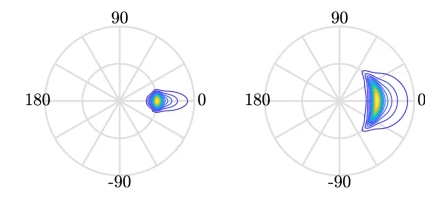
When it is very windy or storms pass-over large sea areas, surface waves grow from short choppy wind-sea waves into powerful swell waves. The height and energy of the waves is larger in winter time, when there are more storms. wind-sea waves have short wavelengths / wave periods (like ripples) while swell waves have longer periods (at a lower frequency).
The example file contains a obervations of sea temperatures, and waves properties at different buoys around the UK.
The dataset is stored as a .csv file: each row holds information for a
single wave buoy, and the columns represent:
| Column | Description |
|---|---|
| record_id | Unique id for the observation |
| buoy_id | Unique id for the wave buoy |
| Name | Name of the wave buoy |
| Date | Date & time of measurement in day/month/year hour:minute |
| Tz | The average wave period (in seconds) |
| Peak Direction | The direction of the highest energy waves (in degrees) |
| Tpeak | The period of the highest energy waves (in seconds) |
| Wave Height | Significant* wave height (in metres) |
| Temperature | Water temperature (in degrees C) |
| Spread | The “directional spread” at Tpeak (in degrees) |
| Operations | Sea safety classification |
| Seastate | Categorised by period |
| Quadrant | Categorised by prevailing wave direction |
* “significant” here is defined as the mean wave height (trough to crest) of the highest third of the waves
The first few rows of our first file look like this:
record_id,buoy_id,Name,Date,Tz,Peak Direction,Tpeak,Wave,Height,Temperature,Spread,Operations,Seastate,Quadrant
1,14,SW Isles of Scilly WaveNet Site,17/04/2023,00:00,7.2,263,10,1.8,10.8,26,crew,swell,west
2,7,Hayling Island Waverider,17/04/2023,00:00,4,193,11.1,0.2,10.2,14,crew,swell,south
3,5,Firth of Forth WaveNet Site,17/04/2023,00:00,3.7,115,4.5,0.6,7.8,28,crew,windsea,east
4,3,Chesil Waverider,17/04/2023,00:00,5.5,225,8.3,0.5,10.2,48,crew,swell,south
5,10,M6 Buoy,17/04/2023,00:00,7.6,240,11.7,4.5,11.5,89,no,go,swell,west
6,9,Lomond,17/04/2023,00:00,4,NaN,NaN,0.5,NaN,NaN,crew,swell,north
About Libraries
A library in Python contains a set of tools (called functions) that perform tasks on our data. Importing a library is like getting a piece of lab equipment out of a storage locker and setting it up on the bench for use in a project. Once a library is set up, it can be used or called to perform the task(s) it was built to do.
Pandas in Python
One of the best options for working with tabular data in Python is to use the Python Data Analysis Library (a.k.a. Pandas). The Pandas library provides data structures, produces high quality plots with matplotlib and integrates nicely with other libraries that use NumPy (which is another Python library) arrays.
Python doesn’t load all of the libraries available to it by default. We have to
add an import statement to our code in order to use library functions. To import
a library, we use the syntax import libraryName. If we want to give the
library a nickname to shorten the command, we can add as nickNameHere. An
example of importing the pandas library using the common nickname pd is below.
import pandas as pd
Each time we call a function that’s in a library, we use the syntax
LibraryName.FunctionName. Adding the library name with a . before the
function name tells Python where to find the function. In the example above, we
have imported Pandas as pd. This means we don’t have to type out pandas each
time we call a Pandas function.
Reading CSV Data Using Pandas
We will begin by locating and reading our wave data which are in CSV format. CSV stands for
Comma-Separated Values and is a common way to store formatted data. Other symbols may also be used, so
you might see tab-separated, colon-separated or space separated files. It is quite easy to replace
one separator with another, to match your application. The first line in the file often has headers
to explain what is in each column. CSV (and other separators) make it easy to share data, and can be
imported and exported from many applications, including Microsoft Excel. For more details on CSV
files, see the Data Organisation in Spreadsheets lesson.
We can use Pandas’ read_csv function to pull the file directly into a DataFrame.
So What’s a DataFrame?
A DataFrame is a 2-dimensional data structure that can store data of different
types (including characters, integers, floating point values, factors and more)
in columns. It is similar to a spreadsheet or an SQL table or the data.frame in
R. A DataFrame always has an index (0-based). An index refers to the position of
an element in the data structure.
# Note that pd.read_csv is used because we imported pandas as pd
pd.read_csv("data/waves.csv")
Referring to libraries
If you import a library using its full name, you need to use that name when using functions from it. If you use a nickname, you can only use the nickname when calling functions from that library For example, if you use
import pandas, you would need to writepandas.read_csv(...), but if you useimport pandas as pd, writingpandas.read_csv(...)will show an error ofname 'pandas' is not defined
The above command yields the output below:
,record_id,buoy_id,Name,Date,Tz,Peak Direction,Tpeak,Wave Height,Temperature,Spread,Operations,Seastate,Quadrant
0,1,14,SW Isles of Scilly WaveNet Site,17/04/2023 00:00,7.2,263.0,10.0,1.80,10.80,26.0,crew,swell,west
1,2,7,Hayling Island Waverider,17/04/2023 00:00,4.0,193.0,11.1,0.20,10.20,14.0,crew,swell,south
2,3,5,Firth of Forth WaveNet Site,17/04/2023 00:00,3.7,115.0,4.5,0.60,7.80,28.0,crew,windsea,east
3,4,3,Chesil Waverider,17/04/2023 00:00,5.5,225.0,8.3,0.50,10.20,48.0,crew,swell,south
4,5,10,M6 Buoy,17/04/2023 00:00,7.6,240.0,11.7,4.50,11.50,89.0,no go,swell,west
...,...,...,...,...,...,...,...,...,...,...,...,...,...
2068,2069,16,west of Hebrides,18/10/2022 16:00,6.1,13.0,9.1,1.46,12.70,28.0,crew,swell,north
2069,2070,16,west of Hebrides,18/10/2022 16:30,5.9,11.0,8.7,1.49,12.70,34.0,crew,swell,north
2070,2071,16,west of Hebrides,18/10/2022 17:00,5.6,3.0,9.5,1.36,12.65,34.0,crew,swell,north
2071,2072,16,west of Hebrides,18/10/2022 17:30,5.7,347.0,10.0,1.39,12.70,31.0,crew,swell,north
2072,2073,16,west of Hebrides,18/10/2022 18:00,5.7,8.0,8.7,1.36,12.65,34.0,crew,swell,north
2073 rows × 13 columns
We can see that there were 2073 rows parsed. Each row has 13
columns. The first column is the index of the DataFrame. The index is used to
identify the position of the data, but it is not an actual column of the DataFrame
(but note that in this instance we also have a record_id which is the same as the index, and
is a column of the DataFrame).
It looks like the read_csv function in Pandas read our file properly. However,
we haven’t saved any data to memory so we can work with it. We need to assign the
DataFrame to a variable. Remember that a variable is a name for a value, such as x,
or data. We can create a new object with a variable name by assigning a value to it using =.
Let’s call the imported wave data waves_df:
waves_df = pd.read_csv("data/waves.csv")
Notice when you assign the imported DataFrame to a variable, Python does not
produce any output on the screen. We can view the value of the waves_df
object by typing its name into the Python command prompt.
waves_df
which prints contents like above.
Note: if the output is too wide to print on your narrow terminal window, you may see something slightly different as the large set of data scrolls past. You may see simply the last column of data. Never fear, all the data is there, if you scroll up.
If we selecting just a few rows, so it is easier to fit on one window, you can see that pandas has neatly formatted the data to fit our screen:
waves_df.head() # The head() method displays the first several lines of a file. It is discussed below.
,record_id,buoy_id,Name,Date,Tz,Peak Direction,Tpeak,Wave Height,Temperature,Spread,Operations,Seastate,Quadrant
0,1,14,SW Isles of Scilly WaveNet Site,17/04/2023 00:00,7.2,263.0,10.0,1.80,10.80,26.0,crew,swell,west
1,2,7,Hayling Island Waverider,17/04/2023 00:00,4.0,193.0,11.1,0.20,10.20,14.0,crew,swell,south
2,3,5,Firth of Forth WaveNet Site,17/04/2023 00:00,3.7,115.0,4.5,0.60,7.80,28.0,crew,windsea,east
3,4,3,Chesil Waverider,17/04/2023 00:00,5.5,225.0,8.3,0.50,10.20,48.0,crew,swell,south
4,5,10,M6 Buoy,17/04/2023 00:00,7.6,240.0,11.7,4.50,11.50,89.0,no go,swell,west
Exploring Our Wave Buoy Data
Again, we can use the type function to see what kind of thing waves_df is:
type(waves_df)
<class 'pandas.core.frame.DataFrame'>
As expected, it’s a DataFrame (or, to use the full name that Python uses to refer
to it internally, a pandas.core.frame.DataFrame).
What kind of things does waves_df contain? DataFrames have an attribute
called dtypes that answers this:
waves_df.dtypes
record_id           int64
buoy_id             int64
Name               object
Date               object
Tz                float64
Peak Direction    float64
Tpeak             float64
Wave Height       float64
Temperature       float64
Spread            float64
Operations         object
Seastate           object
Quadrant           object
dtype: object
All the values in a column have the same type. For example, buoy_id have type
int64, which is a kind of integer. Cells in the buoy_id column cannot have
fractional values, but the TPeak and Wave Height columns can, because they
have type float64. The object type doesn’t have a very helpful name, but in
this case it represents strings (such as ‘swell’ and ‘windsea’ in the case of Seastate).
We’ll talk a bit more about what the different formats mean in a different lesson.
Useful Ways to View DataFrame Objects in Python
There are many ways to summarize and access the data stored in DataFrames, using attributes and methods provided by the DataFrame object.
To access an attribute, use the DataFrame object name followed by the attribute
name df_object.attribute. Using the DataFrame waves_df and attribute
columns, an index of all the column names in the DataFrame can be accessed
with waves_df.columns.
Methods are called in a similar fashion using the syntax df_object.method().
As an example, waves_df.head() gets the first few rows in the DataFrame
waves_df using the head() method. With a method we can supply extra
information in the parens to control behaviour.
Let’s look at the data using these.
Challenge - DataFrames
Using our DataFrame
waves_df, try out the attributes & methods below to see what they return.
waves_df.columns
waves_df.shapeTake note of the output ofshape- what format does it return the shape of the DataFrame in? HINT: More on tuples herewaves_df.head()Also, what doeswaves_df.head(15)do?waves_df.tail()
Calculating Statistics From Data In A Pandas DataFrame
We’ve read our data into Python. Next, let’s perform some quick summary statistics to learn more about the data that we’re working with. We might want to know how many observations were collected in each site, or how many observations were made at each named buoy. We can perform summary stats quickly using groups. But first we need to figure out what we want to group by.
Let’s begin by exploring our data:
# Look at the column names
waves_df.columns
which returns:
Index(['record_id', 'buoy_id', 'Name', 'Date', 'Tz', 'Peak Direction', 'Tpeak',
       'Wave Height', 'Temperature', 'Spread', 'Operations', 'Seastate',
       'Quadrant'],
      dtype='object')
Let’s get a list of all the buoys. The pd.unique function tells us all of
the unique values in the Name column.
pd.unique(waves_df['Name'])
which returns:
array(['SW Isles of Scilly WaveNet Site', 'Hayling Island Waverider',
       'Firth of Forth WaveNet Site', 'Chesil Waverider', 'M6 Buoy',
       'Lomond', 'Cardigan Bay', 'South Pembrokeshire WaveNet Site',
       'Greenwich Light Vessel', 'west of Hebrides'], dtype=object)
Challenge - Statistics
Create a list of unique site IDs (“buoy_id”) found in the waves data. Call it
buoy_ids. How many unique sites are there in the data? How many unique buoys are in the data?What is the difference between using
len(buoy_id)andwaves_df['buoy_id'].nunique()? in this case, the result is the same but when might be the difference be important?
Groups in Pandas
We often want to calculate summary statistics grouped by subsets or attributes within fields of our data. For example, we might want to calculate the average Wave Height at all buoys per Seastate.
We can calculate basic statistics for all records in a single column using the syntax below:
waves_df['Temperature'].describe()
which gives the following
count    1197.000000
mean       12.872891
std         4.678751
min         5.150000
25%        12.200000
50%        12.950000
75%        17.300000
max        18.700000
Name: Temperature, dtype: float64
What counts don’t include
Note that the value of
countis not the same as the total number of rows. This is because statistical methods in Pandas ignore NaN (“not a number”) values. We can count the total number of of NaNs usingwaves_df["Temperature"].isna().sum(), which returns 876. 876 + 1197 is 2073, which is the total number of rows in the DataFrame
We can also extract one specific metric if we wish:
waves_df['Temperature'].min()
waves_df['Temperature'].max()
waves_df['Temperature'].mean()
waves_df['Temperature'].std()
waves_df['Temperature'].count()
But if we want to summarize by one or more variables, for example Seastate, we can
use Pandas’ .groupby method. Once we’ve created a groupby DataFrame, we
can quickly calculate summary statistics by a group of our choice.
# Group data by Seastate
grouped_data = waves_df.groupby('Seastate')
The Pandas describe function will return descriptive stats including: mean,
median, max, min, std and count for a particular column in the data. Pandas’
describe function will only return summary values for columns containing
numeric data (does this always make sense?)
# Summary statistics for all numeric columns by Seastate
grouped_data.describe()
# Provide the mean for each numeric column by Seastate
grouped_data.mean()
grouped_data.mean() produces
record_id,buoy_id,...,Temperature,Spread
,count,mean,std,min,25%,50%,75%,max,count,mean,...,75%,max,count,mean,std,min,25%,50%,75%,max
Seastate,
swell,1747.0,1019.925587,645.553036,1.0,441.50,878.0,1636.5,2073.0,1747.0,11.464797,...,17.4000,18.70,378.0,30.592593,10.035383,14.0,23.0,28.0,36.0,89.0
windsea,326.0,1128.500000,188.099299,3.0,1036.25,1121.5,1273.5,1355.0,326.0,7.079755,...,12.4875,13.35,326.0,25.036810,9.598327,9.0,16.0,25.0,31.0,68.0
2 rows × 64 columns
The groupby command is powerful in that it allows us to quickly generate
summary stats.
This example shows that the wave height associated with water described as ‘swell’ is much larger than the wave heights classified as ‘windsea’.
Challenge - Summary Data
- How many records have the prevailing wave direction (Quadrant) ‘north’ and how many ‘west’?
- What happens when you group by two columns using the following syntax and then calculate mean values?
grouped_data2 = waves_df.groupby(['Seastate', 'Quadrant'])grouped_data2.mean()- Summarize Temperature values for swell and windsea states in your data.
Solution to 3
waves_df.groupby(['Seastate'])["Temperature"].describe()which produces the following:
            count    mean         std         min     25%      50%      75%        max
Seastate
   swell    871.0    14.703502    3.626322    5.15    12.75    17.10    17.4000    18.70
 windsea    326.0    7.981902     3.518419    5.15     5.40     5.45    12.4875    13.35
Quickly Creating Summary Counts in Pandas
Let’s next count the number of records for each buoy. We can do this in a few
ways, but we’ll use groupby combined with a count() method.
# Count the number of samples by Name
name_counts = waves_df.groupby('Name')['record_id'].count()
print(name_counts)
Or, we can also count just the rows that have the Name “SW Isle of Scilly WaveNet Site”:
waves_df.groupby('Name')['record_id'].count()['SW Isles of Scilly WaveNet Site']
Basic Maths Functions
If we wanted to, we could perform maths on an entire column of our data. For example let’s convert all the degrees values to radians.
# convert the directions from degrees to radians
# Sometimes people use different units for directions, for example we could describe
# the directions in terms of radians (where a full circle 360 degrees = 2*pi radians)
# To do this we need to use the math library which contains the constant pi

# Convert degrees to radians by multiplying all direction values values by pi/180
import math # the constant pi is stored in the math(s) library, so need to import it
waves_df['Peak Direction'] * math.pi / 180
Constants
It is normal for code to include variables that have values that should not change, for example. the mathematical value of pi. These are called constants. The maths library contains three numerical constants: pi, e, and tau, but other built-in modules also contain constants. The
oslibrary (which provides a portable way of using operating system tools, such as creating directories) lists error codes as constants, while thecalendarlibrary contains the days of the week mapped to numerical index (from monday as zero) as constants.The convention for naming constants is to use block capitals (n.b.
math.pidoesn’t follow this!) and to list them all together at the top of a module.
Challenge - maths & formatting
Convert the temperature colum to Kelvin (adding 273.15 to every value), and round the answer to 1 decimal place
Solution
(waves_df["Temperature"] + 273.15).round(1)
Challenge - normalising values
Sometimes, we need to normalise values. A common way of doing this is to scale values between 0 and 1, using
y = (x - min) / (max - min). Using this equation, scale the Temperature columnSolution
x = waves_df["Temperature"]
y = (x - x.min()) / (x.max() - x.min())
A more practical use of this might be to normalize the data according to a mean, area, or some other value calculated from our data.
Key Points
Libraries enable us to extend the functionality of Python.
Pandas is a popular library for working with data.
A Dataframe is a Pandas data structure that allows one to access data by column (name or index) or row.
Aggregating data using the
groupby()function enables you to generate useful summaries of data quickly.Plots can be created from DataFrames or subsets of data that have been generated with
groupby().
Working with netCDF files and creating animations
Overview
Teaching: 90 min
Exercises: 0 minQuestions
How can we work with netCDF files (often used in Earth science)?
How can we create maps with coastlines?
How do we create lots of figures at once?
How can we create animations to help with visualisation?
How can we work with datetimes in Python?
Objectives
Learn how to use Python’s netCDF4 and Cartopy libraries
Learn how to work with datetime objects
Learn how to create animated plots
NetCDF files
What about data stored in other types of files? Scientific data is often stored in NetCDF files.
NetCDFs are nice! They are self-describing - i.e. they are set up to contain both the data required, and any metadata that helps the user understand that data. They are often used to store large 3 (or greater) dimensional matrices or tensors, making them ideal for storing data on e.g. the vertical and horizontal structure of the atmosphere over long timescales.
Data such as the ERA5 climatological reanalysis are stored in netCDF - often with tens or hundreds of different atmospheric variables gridded at each temporal and spatial point.
Such large datasets would be very unwieldy to work with in Numpy or even using Pandas, but netCDF has us covered. We will be looking a less complex dataset than this here - but the principles can be applied to using these datasets also.
Python has a library called netCDF4 which is designed for operating with these files.
We will here use data from the Climate Research Unit at the UEA, describing monthly-mean global surface temperature.
Using other libraries
For the rest of this lesson, we need to use a python library that isn’t included in the default installation of Anaconda. There are various ways to doing this, depending on how you opened the Jupyter Notebook:
If you’re using Anaconda Navigator:
- return to the main window of Anaconda Navigator
- select “Environments” from the left-hand menu, and then “base (root)”
- Select the Not Installed filter option to list all packages that are available in the environment’s channels, but not installed.
- Select the name of the package you want to install. We want
NetCDF4- Click Apply
If you opened the Jupyter Notebook via the command line:
- you’ll need to close the Notebook (Ctrl+C, twice)
- run the command
conda install netcdf4, and accept any prompt(s) (y)
import netCDF4 as nc
We can then import a netCDF file, and check to see what python thinks its type is:
globaldata = nc.Dataset("cru_data.nc")
print(type(globaldata))
<class 'netCDF4._netCDF4.Dataset'>
We can look at what variables our netCDF contains by doing:
globaldata.variables.keys()
dict_keys(['lon', 'lat', 'time', 'tmp', 'stn'])
Here we can infer that we have three co-ordinates, longitude, latitude and time, and two variables ‘tmp’ and ‘stn’. We can probably guess that ‘tmp’ is temperature, since we are looking at surface temperature data, but what is ‘stn’? Let’s check this out in more detail. We can do this using:
globaldata.variables['stn']
<class 'netCDF4._netCDF4.Variable'>
int32 stn(time, lat, lon)
    description: number of stations contributing to each datum
unlimited dimensions: time
current shape = (84, 360, 720)
filling on, default _FillValue of -2147483647 used
So we see that ‘stn’ is some extra data that is useful to understand the reliability of our temperature data. We can also see the shape of the data - (84, 360, 720). This gives us an indication of the co-ordinates - it is likely that 360 and 720 refer to latitude/longitude, which means we have 84 temporal points. Let’s check using the .variables['var'] syntax again:
globaldata.variables['time']
<class 'netCDF4._netCDF4.Variable'>
float32 time(time)
    long_name: time
    units: days since 1900-1-1
    calendar: gregorian
unlimited dimensions: time
current shape = (84,)
filling on, default _FillValue of 9.969209968386869e+36 used
Yes, this checks out. Our time array has a length of 84. But what does “days since 1900-1-1” mean for us? Let’s have a look at the actual values in the dataset. We do this by adding a slice to what we put previously. Let’s slice for all of the data in the array.
globaldata.variables['time'][:]
masked_array(data=[40557., 40587., 40616., 40647., 40677., 40708., 40738.,
                   40769., 40800., 40830., 40861., 40891., 40922., 40952.,
                   40982., 41013., 41043., 41074., 41104., 41135., 41166.,
                   41196., 41227., 41257., 41288., 41318., 41347., 41378.,
                   41408., 41439., 41469., 41500., 41531., 41561., 41592.,
                   41622., 41653., 41683., 41712., 41743., 41773., 41804.,
                   41834., 41865., 41896., 41926., 41957., 41987., 42018.,
                   42048., 42077., 42108., 42138., 42169., 42199., 42230.,
                   42261., 42291., 42322., 42352., 42383., 42413., 42443.,
                   42474., 42504., 42535., 42565., 42596., 42627., 42657.,
                   42688., 42718., 42749., 42779., 42808., 42839., 42869.,
                   42900., 42930., 42961., 42992., 43022., 43053., 43083.],
             mask=False,
       fill_value=1e+20,
            dtype=float32)
We could similarly do so for an arbitrary index, let’s say the first one:
globaldata.variables['time'][0]
masked_array(data=40557.,
             mask=False,
       fill_value=1e+20,
            dtype=float32)
masked_array(data=40557.,
             mask=False,
       fill_value=1e+20,
            dtype=float32)
So our time data is a set of numbers, differing by 30 or 31. These must be monthly data then! But how can we get this into a nice format? It seems complicated! Let’s put this to one side and focus more on our temperature data. Let’s say we were just interested in a particular region. To do this, we can slice across the array like we would with any Numpy array:
import numpy as np
sliced = globaldata.variables['tmp'][:, 10:20, 30:40]
np.shape(sliced)
(84, 10, 10)
A useful thing to do whenever working with data is to plot it up! So let’s do just that. We load in our long/lat data (x and y, opposite way round to how we normally think about lat/long!), our temperature data at our first timestep, define a number of gradations in the contour (how many colour levels), and a colour map. Since we’re using temperature, let’s use the ‘Reds’ colourmap. More examples can be found here.
from matplotlib import pyplot as plt # best practice is to put imports at the top of the file

lon = globaldata.variables['lon'][:]
lat = globaldata.variables['lat'][:]
days_since_1Jan1900 = globaldata.variables['time'][:]
tmp = globaldata.variables['tmp'][:]

fig = plt.figure()
plt.contourf(lon, lat, tmp[0], 16, cmap='Reds')
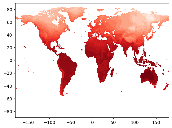
This looks good! We seem to have a map of surface temperature - this looks like what the Earth’s surface should look like! But we have only plotted up one timestep here, which is not useful for looking at the whole dataset. And what if we want to look at a specific region, or use a different projection?
For this, we will introduce another library, cartopy. Cartopy is a staple library for Earth scientists, as it provides a way of creating nice map-based figures.
We will do the same as we did before - close our Jupyter notebook, install cartopy, and then re-open it. Follow the same steps as before, but using conda install cartopy (via command line), or using the Navigator. I recommend trying it this time with the command line - it is better to get used to using it now rather than later as it is very powerful!
Now, let’s create a map! We’ll start by importing cartopy:
import cartopy
Let’s define a map projection to begin with. We will start using the simplest - just plotting things on a lat/long grid with no transformation - the PlateCarree projection. We then need to interface cartopy with our matplotlib Figure, we need to define an Axes object, and connect it with our map projection. Thankfully, the Axes object has an argument that lets us do this quickly. Finally, let’s draw the coastlines in - using the coastlines method. This method is available to use thanks to our use of our projection proj. Let’s do this on an empty plot to begin with.
plt.figure()
proj = cartopy.crs.PlateCarree()
ax = plt.axes(projection=proj)
ax.coastlines()
plt.show()

Now put this together with our contour data:
plt.figure()
proj = cartopy.crs.PlateCarree()
ax = plt.axes(projection=proj) # this has to come before we do our contour else it will overlay the empty coastlines plot on top!
plt.contourf(lon, lat, tmp[0], 16, cmap='Reds')
ax.coastlines()
plt.show()

This looks nice - but we can do a lot more with this. What if we want to look with a different projection? Let’s try changing proj to everyone’s favourite Mercator projection (a full list of Cartopy map projections can be found here).
plt.figure()
proj = cartopy.crs.Mercator()
ax = plt.axes(projection=proj) # this has to come before we do our contour else it will overlay the empty coastlines plot on top!
plt.contourf(lon, lat, tmp[0], 16, cmap='Reds')
ax.coastlines()
plt.show()

Our coastlines have disappeared? This is because our contour data is not being transformed to account for our changed projection. This thankfully is not too painful to resolve; we can use the transform argument of contourf to do this. We use PlateCarree as our transform here, and Cartopy will handle the rest.
plt.figure()
proj = cartopy.crs.Mercator()
ax = plt.axes(projection=proj) # this has to come before we do our contour else it will overlay the empty coastlines plot on top!
plt.contourf(lon, lat, tmp[0], 16, cmap='Reds', transform=ccrs.PlateCarree())
ax.coastlines()
plt.show()

Now it works! We can see that the contour data has warped to match the changed coastlines. This approach works for other, more complex projections also. Let’s try looking at a specific region then. There are two ways to do this. First is to slice our array as we did earlier, and just plot that data. This is the more efficient way to do things - particularly with large datasets. We can also cheat a little bit, and just plot a specific region of the whole dataset using ax.set_extent. This has the benefit of letting us use lat/long directly, rather than having to do the conversion ourselves when slicing the array:
ax.set_extent([-5.5, -2.5, 51, 54], crs=cartopy.crs.PlateCarree()) # pick out Wales!
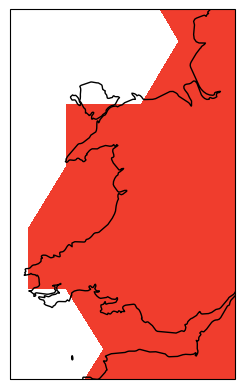
Ok, it looks like our data is far too low resolution to work with on scales as small as Wales. Let’s try thinking about making our initial global map into a nice, high quality figure. We should first do what any good scientists do and label our axes and write a title. We do this using the xlabel/ylabel functions, and we can draw in labelled gridlines on our map using gridlines with draw_labels = True (again this is a nice feature of Cartopy that lets us do this). We also switch back to a more sensible map projection.
plt.figure()
proj = cartopy.crs.PlateCarree()
ax = plt.axes(projection=proj) # this has to come before we do our contour else it will overlay the empty coastlines plot on top!
plt.contourf(lon, lat, tmp[0], 16, cmap='Reds', transform=cartopy.crs.PlateCarree())
ax.coastlines()
plt.xlabel('Longitude')
plt.ylabel('Latitude')
ax.gridlines(draw_labels=True)

plt.title('Surface Temperature (°C)')
plt.show()

Now we can add a colour bar in so that our data is actually meaningful. This can be done via:
plt.colorbar(orientation = 'horizontal')
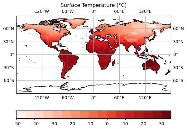
We now have a plot that we could realistically put into a paper! However, we are still only looking at individual timesteps here. And we aren’t any closer to being able to convert our days_since_1Jan1900 variable into a nicely formatted date - this would be really useful for our figure title if we could!
We could use a for loop, to generate several of these plots all at once. This is perfectly reasonable to do, particularly if we need still images of specific timesteps. We could do something like:
plt.figure()
proj = cartopy.crs.PlateCarree()
for idx, val in enumerate(tmp):
    ax = plt.axes(projection=proj) # this has to come before we do our contour else it will overlay the empty coastlines plot on top!

    plt.contourf(lon, lat, val, 16, cmap='Reds', transform=cartopy.crs.PlateCarree())
    ax.coastlines()
    plt.xlabel('Longitude')
    plt.ylabel('Latitude')
    ax.gridlines(draw_labels=True)

    plt.title(f'Surface Temperature (°C)')
    plt.colorbar(orientation = 'horizontal')
    plt.save(f'surface_temperature_{idx}.png)
A couple of things here. We use plt.save to save our figure instead of printing it to screen. This is useful as it means you can generate lots of figures and save them without having to do so manually! We need to use unique filenames each time though. We use idx for this. Notice how we used {} to format it? This is because of the little f before we start the string. This is a feature in Python called an f-string, which stands for formatted string. These are exceptionally useful - allowing you to use variables in strings in a quick and simple way.
What if we want to visualise our data however? Or if we want to present it in an intuitive way in a presentation or blog post? A slicker way of doing this is by creating an animation. This used to be very complex, but has got easier over time as Python has developed further. We will do this using the animation sub-library of matplotlib - in particular using a FuncAnimation.
from matplotlib import animation
anim = animation.FuncAnimation(fig, animate,
                            frames = 10,
                            interval = 500,
                            )
FuncAnimation reads in a base Figure, a function animate that updates the figure, a number of frames we want to animate, and an interval between each frame (in milliseconds, so smaller = faster).
We therefore need to write a function to handle the updating of the figure! We have all of the code needed already pretty much.
def animate_figure(frame):
    data = tmp[frame]
    plt.contourf(lon, lat, data, 16, cmap='Reds', transform=ccrs.PlateCarree(),
            levels = np.linspace(vmin, vmax, 41), vmin = vmin, vmax = vmax)
    plt.xlabel('Longitude')
    plt.ylabel('Latitude')
    plt.title('Surface Temperature (°C), {get_date(idx)}')
FuncAnimation will handle the for loop for us here - we need to supply the function and it will loop frames times through our dataset.
Let’s check it out! We’ll keep frames at 10, with a delay of 100 milliseconds.
def animate_figure(frame):
    data = tmp[frame]
    plt.contourf(lon, lat, data, 16, cmap='Reds', transform=ccrs.PlateCarree(),
            levels = np.linspace(vmin, vmax, 41), vmin = vmin, vmax = vmax)
    plt.xlabel('Longitude')
    plt.ylabel('Latitude')
    plt.title('Surface Temperature (°C)')

tmp = globaldata.variables['tmp'][:]

fig = plt.figure()
proj = cartopy.crs.PlateCarree()

ax = plt.axes(projection=proj)
ax.coastlines()
ax.gridlines(draw_labels=True)

from matplotlib import animation

anim = animation.FuncAnimation(fig, animate_figure,
                            frames = 10,
                            interval = 100,
                            )

anim.save('CRU_data_anim.gif')
You’ll notice we haven’t included the colour bar here. This is because this requires a bit more thought. We want our colour bar to be consistent. But this means that we need to make sure that the data match this colour bar at every time step! Currently, the deepest red and the brightest white are set to the extreme ranges of whatever temperature data we display at each timestep. We can fix this by ensuring that the contour data and the colour bar are normalised to the highest and lowest points in our temperature dataset.
Note that this approach doesn't always work! If your data has large outliers in it, you will need to clean these up first else the vast majority of your colours will be in a very narrow range.
We start by taking the smallest and largest temperature data in our tmp dataset. We can then use the vmin and vmax keywords of the contourf function - this will effectively set the max and min colours to this value (which are the largest and smallest in the dataset) - forcing consistency across time periods. We do the same for the colour bar also. This means we don’t need to update the colour bar every frame - it is consistent for every timestep so we can just define it before we start the animation! We will create a plot at time 0, so that the colour bar can be made without throwing an error.
vmin = np.min(tmp)
vmax = np.max(tmp)

def animate_figure(frame):
    data = tmp[frame]
    plt.contourf(lon, lat, data, 16, cmap='Reds', transform=ccrs.PlateCarree(),
            levels = np.linspace(vmin, vmax, 41), vmin = vmin, vmax = vmax)
    plt.xlabel('Longitude')
    plt.ylabel('Latitude')
    plt.title('Surface Temperature (°C)')

tmp = globaldata.variables['tmp'][:]

fig = plt.figure()
proj = cartopy.crs.PlateCarree()

ax = plt.axes(projection=proj)
ax.coastlines()
ax.gridlines(draw_labels=True)

plt.contourf(lon, lat, tmp[0], 16, cmap='Reds', transform=ccrs.PlateCarree(),
        levels = np.linspace(vmin, vmax, 41), vmin = vmin, vmax = vmax)

plt.colorbar(orientation = 'horizontal')

from matplotlib import animation

anim = animation.FuncAnimation(fig, animate_figure,
                            frames = 10,
                            interval = 100,
                            )

anim.save('CRU_data_anim.gif')

Nearly there! Two things stand out here. The first of which is that the colour bar now has some rather unfortunate tick labels. The second is that we still don’t have a means of knowing when each data point occurs in time! Let’s fix the first thing first. We can do this using the ticks argument of colorbar:
plt.colorbar(orientation = 'horizontal', ticks = np.arange(-50, 50, 10))
Now let’s finally use our date data! There is a convenient way to work with date variables in Python - the datetime library. Let’s write this into a function, so we can re-use it later. It also makes the code a bit easier to read. We have our input data in days since 1st January 1900. The datetime module has a neat function called timedelta. This lets us effectively look at the difference between our date and another given date (it can also do this for time, down to microsecond resolution!). datetime.date gives us a date in YYYY-MM-DD format. The magic of timedelta lets us add our current date to 1900-01-01 to get the date we need!
import datetime

def get_date(idx):
    date = datetime.date(1900, 1, 1) + datetime.timedelta(days=int(days_since_1Jan1900[idx]))
    print(f'date = {date}')
get_date(0)
datetime.date(2011, 1, 16)
We are almost at what we want. We have the correct date now (16 Jan 2011), but want it in a format we can display nicely. For this, we use strftime (string formatting for time). This is a method of the date object, and takes in a format string as an argument. This lets us specify how we want to display the date - let’s just pick the month and year here since we are dealing with monthly data. A cheat sheet for this (mapping format string -> output type) can be found here.
import datetime

def get_date(idx):

    date = datetime.date(1900, 1, 1) + datetime.timedelta(days=int(days_since_1Jan1900[idx]))
    print(f'date = {date}')
    date_string = date.strftime('%B %Y') # https://strftime.org/ for a cheat sheet
    return date_string
get_date(0)
'January 2011'
Finally, let’s put all this together in our animate_figure function! Note the use of an f-string again in plt.title. We call our get_date function directly here - it will put the output of that function (what it returns) into our title.
vmin = np.min(tmp)
vmax = np.max(tmp)

def get_date(idx):
    date = datetime.date(1900, 1, 1) + datetime.timedelta(days=int(days_since_1Jan1900[idx]))
    print(f'date = {date}')
    date_string = date.strftime('%B %Y') # https://strftime.org/ for a cheat sheet
    return date_string

def animate_figure(frame):
    data = tmp[frame]
    plt.contourf(lon, lat, data, 16, cmap='Reds', transform=ccrs.PlateCarree(),
            levels = np.linspace(vmin, vmax, 41), vmin = vmin, vmax = vmax)
    plt.xlabel('Longitude')
    plt.ylabel('Latitude')
    plt.title(f'Surface Temperature (°C), {get_date(frame)}')

tmp = globaldata.variables['tmp'][:]

fig = plt.figure()

proj = cartopy.crs.PlateCarree()

ax = plt.axes(projection=proj)
ax.coastlines()
ax.gridlines(draw_labels=True)

plt.contourf(lon, lat, tmp[0], 16, cmap='Reds', transform=ccrs.PlateCarree(),
        levels = np.linspace(vmin, vmax, 41), vmin = vmin, vmax = vmax)

plt.colorbar(orientation = 'horizontal', ticks = np.arange(-50, 50, 10))

from matplotlib import animation

anim = animation.FuncAnimation(fig, animate_figure,
                            frames = 84,
                            interval = 100,
                            )

anim.save('CRU_data_anim.gif')

This looks good now! Now we have the date on the plots, we can see that it makes intuitive sense - the temperature is lower in the Northern Hemisphere during Northern Hemisphere Winter, and vice versa.
Key Points
Python’s netCDF4, datetime and cartopy libraries are really useful for working with gridded Earth science data
We can use matplotlib to create animations using functions
Next steps
Overview
Teaching: 40 min
Exercises: 0 minQuestions
Where can I go from here?
What are some useful tips and tricks to know when coding?
What other opportunities are available for me to learn more?
Objectives
Knowing what best practices are when thinking about code (as opposed to just writing it!)
Determine where additional training materials can be found.
Things to try and think about when writing code
-
Coding is difficult!
If you get stuff wrong, that’s OK! You will 100% write code that doesn’t work, or has bugs in it. This is normal! I’ve been writing code in Python for 10 years and still get basic stuff wrong.
-
Don’t get discouraged!
The best thing to do is to have a go at solving the problem. Worst case - your code throws an error. Think about what is causing the error, solve it, and move onto the next one! Each time you solve an error, you will know what to do when it occurs again next time. See fixing problems as an opportunity for growth rather than something negative.
-
Break down problems into smaller ones
Think like a scientist - if we see a big problem, it is often constructive to break it down into several smaller ones, then build them together to find the solution. As tempting as it is to write big long scripts with lots of repeated (read: copy and pasted) code, if you can, don’t! Think about problems before you solve them - how can we decompose it into functions that solve one specific problem each, and then bring it all together?
This can be a huge time saver as well - often you’ll write bits of code that solve similar problems - why not just re-use the same functions/code from your previous project? I have an ever-evolving list of useful functions I’ve written to solve specific (often menial) problems I often face when doing data analysis/visualisation.
-
Think logically/procedurally
Often your code will fail and you’ll be unsure as to why. The computer will only ever execute the actions you write exactly as you have written them. Work through your code and try and work out what is happening to your variables at each step.
-
Be organised
A huge amount of overhead with software is maintenance - in scientific terms this might just mean coming back to code you wrote previously for a paper correction or something. So many times I’ve looked back at my own code and thought “what on Earth is this nonsense!”. Writing logical code split into functions with lots of comments helps readability a ton. Also, use logical names and structures for everything. If your data analysis has a bunch of constants/data imports, keeping these at the top of scripts will help you to work out what they do much easier.
Have different folders for different projects, so that you can navigate to the specific bit of code you were using easier. Name your scripts something meaningful too! You’re not going to remember what “script.py” does in 6 months, but “west_africa_rainfall_analysis.py” might be more useful. This extends to variable names too! Avoid using names like “data” if possible - better to explicitly refer to what you’re looking at (so something like “rainfall_data_in” for loading in a netCDF, then splitting this into variables like “lat”, “long” and “rainfall”).
-
Write comments!
I mentioned this already but its so important it bears repeating - writing comments helps others to understand code you’ve written (without the benefit of having written it), but also helps you to work out what that bit of code you wrote days/weeks/months/years ago does a lot faster than actually reading the code.
Try and have comments both at the top-level (what does this function do/what purpose does it serve?), and also perhaps for individual lines of code for tricks and things that may be a bit arcane to work out without context (e.g. if you are doing some kind of normalisation on your data).
-
Don’t reinvent the wheel!
Often, someone will have already solved the task you want to try and solve. It is often much better to use their solution! Search around for functions that do what you want (Numpy and the scientific computing library Scipy usually have you covered if its anything mathematical), or libraries if your problem is specific to your field of study!
-
Don’t worry about optimisation (yet)
When writing code, premature optimisation is the enemy! Write something that works first, then optimise the bits that are slow. Writing a data analysis script for 100000 different data files? Write something that works for 10 files first, see how fast it is, work out the bits that are slow, then scale. You can always ask me for help if speed is ever an issue. Most data analysis tasks can be run on personal computers. You may eventually run into problems that require High Performance Computing (often abbreviated HPC) - please get in touch if so!
Tips and Tricks
These are some little things which you will likely pick up as you start to write more code, some of which you have seen already. We may not necessarily have used all of these in the earlier portions of the course to minimise cognitive load, but “in the wild” you will likely see people using these!
-
Block comment in Jupyter Notebooks using Ctrl + / (or Cmd + / on Mac)
-
Cut down on typing using the
askeyword…When importing modules, you can use the
askeyword to create a kind of shorthand. For example:import numpy as nplets you typenp.sum(wave_data)instead ofnumpy.sum(wave_data). -
… or using the
fromkeyword.You can also, if you are only importing specific parts of a module, use the
fromkeyword. For example:from netCDF4 import Datasetlets you type
Dataset(wave_data)instead ofnetCDF4.Dataset(wave_data). -
Use
helpto get info on a function (or use Google)e.g.
help(np.sum)(assuming theimport numpy as npsyntax from earlier) -
Use Conda environments!
So far during this course, we have only used the “base” Anaconda environment. An environment is effectively like a fresh install of Python. This can be very useful when working with libraries, as often they will be dependent on other libraries; when one is updated it can cause everything to stop working, or perhaps two different libraries need two different versions of another library to work (often known as “dependency hell”. I tend to use a new Conda environment for each project/application I am working on, as to minimise any conflicts between the stuff I require for each project.
You can create a new Conda environment from the Anaconda Prompt (i.e. command line) using:
conda create --name <your_name_here> python.Or to create one with a specific version of python, in this case an environment called
waves_project:conda create --name waves_project python=3.9.This will create a blank slate Python, from which you can install libraries etc. again (you will need to install Jupyter notebook in this environment if you want to use these, via
conda install jupyter). This is very useful for organising projects, and making sure that your code still works when you revisit it a year later!
Other useful libraries for scientific computing (useful to be aware of, although you likely won’t use some of these until much later)
- Scipy - algorithms for scientific computing - useful for statistics, working with matrices, probability distribution functions, optimisation problems, interpolation/extrapolation and differential equations
- Scikit-image - Image processing
- Scikit-learn - Machine learning/data science - good at almost all standard ML tasks aside from deep learning/neural networks, for which you want to use
TensorFloworPyTorch - BeautifulSoup - web scraping, potentially really useful for data collection
- Dask - parallel computing
- Sympy - symbolic maths using Python! If any of you have used Mathematica, it has similar functionality.
Other languages that might be of interest
- R - also free, focused more on statistics/data manipulation, has similar functionality to Python in a lot of places but may be a little easier to use
- Matlab - University has a paid license, can be good for some specific tasks
- Fortran/C - used by people doing numerical modelling/number crunching, very hard to learn but necessary for some types of computing
- Julia - new upstart language, bridges the gap between the speed of Fortran and the library support/ease of use of Python
Additional training
ARCCA have some training courses available on their website, which I recommend. They tend to run these a few times a year, or you can work through the material in your own time.
ARCCA’s courses (and indeed this one!) are based to various degrees on courses developed by an organisation called The Carpentries. You can find their software lessons here. Additional lessons are available on the Data Carpentries website; these tend to focus on more specific but still potentially relevant things. These are also highly recommended!
Depending on your feedback, I may also offer more advanced courses in future.
Things not covered here (which you may see out in the wild) - read this in your own time if interested!
-
Using the command line
While at first it is useful to run code in Jupyter notebooks or in Spyder, longer term it is very useful to get comfortable using the command line, particularly using the Bash shell (found on Linux/Mac). This will allow you to run your code in batch scripts, allowing for use on HPC systems, or just running lots of iterations of your code at once. ARCCA have some useful training on how to do this.
-
Object oriented code
A lot of code you will see may use what we call an
object orientedapproach. For example, instead of doingnp.sum(array), you may see something similar toarray.sum(). We touched on this when working with our netCDF files - e.g. when loading in a netCDF usingDataset, this is an object, which we operate on using thevariablesmethod to get e.g. our lat/long grids and our temperature fields from the CRU example.This is something I may give a workshop on in future as it is a very useful way of thinking about code when writing your own - particularly for large-scale projects.
Key Points
Write lots of code!
Use the Internet, particularly StackOverflow, use my expertise and talk to one another about problems you are facing!